ORIGINAL ARTICLE
Crack Fault Classification for Planetary
Gearbox Based on Feature Selection Technique
and K-means Clustering Method
Li‑Ming Wang and Yi‑Min Shao
*Abstract
During the condition monitoring of a planetary gearbox, features are extracted from raw data for a fault diagnosis. However, different features have different sensitivity for identifying different fault types, and thus, the selection of a sensitive feature subset from an entire feature set and retaining as much of the class discriminatory information as possible has a directly effect on the accuracy of the classification results. In this paper, an improved hybrid feature selection technique (IHFST) that combines a distance evaluation technique (DET), Pearson’s correlation analysis, and an ad hoc technique is proposed. In IHFST, a temporary feature subset without irrelevant features is first selected according to the distance evaluation criterion of DET, and the Pearson’s correlation analysis and ad hoc technique are then employed to find and remove redundant features in the temporary feature subset, respectively, and hence, a sensitive feature subset without irrelevant or redundant features is selected from the entire feature set. Further, the k‑means clustering method is applied to classify the different kinds of health conditions. The effectiveness of the pro‑ posed method was validated through several experiments carried out on a planetary gearbox with incipient cracks seeded in the tooth root of the sun gear, planet gear, and ring gear. The results show that the proposed method can successfully distinguish the different health conditions of a planetary gearbox, and achieves a better classification performance than other methods. This study proposes a sensitive feature subset selection method that achieves an obvious improvement in terms of the accuracy of the fault classification.
Keywords: Planetary gearbox, Gear crack, Feature selection technique, K‑means classification
© The Author(s) 2018. This article is distributed under the terms of the Creative Commons Attribution 4.0 International License (http://creativecommons.org/licenses/by/4.0/), which permits unrestricted use, distribution, and reproduction in any medium, provided you give appropriate credit to the original author(s) and the source, provide a link to the Creative Commons license, and indicate if changes were made.
1 Introduction
Owing to its advantages of a compact structure, large transmission ratio, and high load capacity, a planetary gear transmission system is widely used in large-scale and complex mechanical equipment [1, 2], e.g., wind tur-bines, helicopters, and automobiles.
A planetary gearbox typically consists of some key components: a sun gear, planet gear, ring gear, carrier, and bearing, and faults may occur in these components owing to fatigue or tough working conditions. Accord-ing to a condition-monitorAccord-ing report on wind turbines, a gearbox failure is the leading contributor to all wind tur-bine failures [3]. A vibration-based method was proven
to be one of the most popular techniques in the fault diagnosis of rotating machinery, and it has been deter-mined that certain changes to the vibration signals can be seen when a fault occurs, e.g., crack or spalling [4–6]. The commonly used vibration signal processing methods can be divided into three categories: time domain methods, frequency domain methods, and time–frequency domain methods. Time domain methods refer to the analysis of a signal with respect to time, and are relatively easy and direct compared to both frequency and time–frequency domain methods. Statistical indicators, the time synchro-nous averaging (TSA) method, and an autoregressive (AR) model are typically used in the fault diagnosis of rotating machinery [4, 7–9]. Frequency domain methods refer to an analysis of the signals with respect to the fre-quency, and a periodic signal in the time domain can be converted into a frequency component through a Fourier
Open Access
*Correspondence: [email protected]
transformation. In this way, researchers can identify the difference between the spectrum of a normal vibration signal and a fault vibration signal with commonly used methods that include a spectrum-based analysis, reso-nance demodulation technique, and cepstrum analysis [10–12]. In contrast, time–frequency domain methods are used to study a signal in both the time and frequency domains simultaneously, allowing both the constituent frequency components and their time variation features to be revealed and analyzed. Researchers have devel-oped various time–frequency domain methods includ-ing a short-time Fourier transformation, Wigner–Ville distribution, continuous wavelet transform, and Hilbert-Huang transformation [13–16]. Although vibration-based methods have been successfully used in the fault diagnosis and condition monitoring of rotating machin-ery, the appearance of faults in the analysis results has to be identified artificially, e.g., the identification of a fault characteristic frequency in the spectrum, the determina-tion of a filter sub-band in a demoduladetermina-tion analysis, or the determination of a wavelet type, all of which require con-siderable of experience and expertise [17–19]. Therefore, it is necessary to develop some intelligent techniques that can automatically determine the health conditions of a planetary gearbox.
Feature extraction is commonly the first important step in an intelligent technique. However, different fea-tures display different sensitivity to fault advancements, and some of the features are redundant or irrelevant to the fault diagnosis or classification result [19–21]. Select-ing a sensitive feature subset and retainSelect-ing as much of the class discriminatory information as possible has a direct effect on the accuracy of the results. Kang et al. [20] developed an outlier-insensitive hybrid feature selection methodology to reduce diagnostic performance deterio-ration caused by outliers in data-driven diagnostics. Peng et al. [22] studied how to select good features according to the maximal statistical dependency criterion based on mutual information. Yang et al. [23] demonstrated an approach to the multi-criteria optimization problem of feature subset selection using a genetic algorithm. Li et al. [24] presented a two-stage feature selection approach combining filter and wrapper techniques to obtain a more compact feature subset for accurate classification of the hybrid faults of a gearbox. Liu et al. [25] introduced a hybrid dimension reduction method that combines kernel feature selection and a kernel Fisher discriminant analysis for a fault-level diagnosis of planetary gearboxes. Lei et al. [19, 26] and Shen et al. [27] proposed a feature subset selection method based on a distance evaluation technique (DET) for fault classification of a roller bearing and gear reducer. Among these feature subset selection methods, DET is relatively simpler and more efficient
than the other methods, and has thus been widely used in fault diagnosis [28–30]. However, DET tends to select redundant features because it does not consider the rela-tionships between features; one relevant feature selected by DET may be redundant in the presence of another relevant feature with which it is strongly correlated. To address this problem, an improved hybrid feature selec-tion technique (IHFST) combining DET, Pearson’s cor-relation analysis, and an ad hoc technique is proposed. Using IHFST, the relevant features are selected accord-ing to the distance evaluation criterion of DET, and the redundant features are then further suppressed based on the Pearson’s correlation analysis and ad hoc technique. Hence, not only irrelevant features, but also redundant features, are removed from the entire feature set based on the proposed IHFST.
Once a sensitive feature subset is selected, it can be classified into several classifications based on some machine learning (ML) methods. The k-means clustering method is a widely used unsupervised pattern recogni-tion algorithm that aims to partirecogni-tion n observations into k clusters, where each observation belongs to the cluster with the nearest mean [31–34]. Therefore, the k-means clustering method is further employed to validate the effectiveness of the proposed IHFST method.
The rest of this paper is organized as follows: Section 2 briefly introduces the feature-subset selection based on DET. Section 3 presents the fault classification process based on the proposed IHFST and k-means method. Sec-tion 4 describes the experiment system and data acqui-sition. The effectiveness of the proposed method as validated using various datasets is then described in Sec-tion 5. Finally, some concluding remarks are provided in Section 6.
2 Brief Review of DET
In fault diagnosis, different features can reflect differ-ent aspects of the vibration properties of the machinery, and certain features are sensitive to certain changes in machine conditions [19–21, 25]. If all features are applied to a fault diagnosis without a careful selection, the com-putation complexity of the algorithm will increase with little gain [26]. Therefore, a feature selection process is necessary to reduce the computation complexity and improve the accuracy of the fault diagnosis. The feature selection process based on DET is briefly introduced.
The basic concept of DET is to measure the ratio of the between-class distance to the within-class distance in the feature vector space, as illustrated in Figure 1, where a high DET value indicates high sensitivity or class separa-bility of the feature.
Suppose that the entire feature set is obtained by
where qi,k,j is the feature value of the jth feature from the ith sample of the kth health condition, Ik is the total sam-ple number of the kth condition, K represents the condi-tion number, and J is the feature number in the feature vector of each sample. The process of informative feature selection based on DET is as follows:
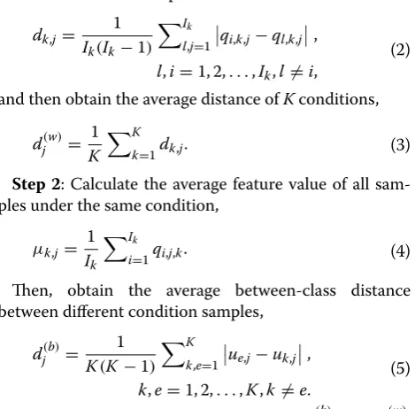
Step 1: Calculate the within-class average distance of
the same condition samples,
and then obtain the average distance of K conditions,
Step 2: Calculate the average feature value of all
sam-ples under the same condition,
Then, obtain the average between-class distance between different condition samples,
Step 3: Calculate the ratio between dj(b) and dj(w),
assigning the compensation factor εj =dj(b)/d(jw), and then normalize it based on the maximum value and obtain the distance evaluation criterion αj=εj/max(εj).
Hence, a feature subset can be selected when the dis-tance evaluation criterion αj is greater than a given threshold. However, the DET method only removes irrel-evant features from the entire feature set. Although the
(1) {qi,k,j, i=1, 2,. . .,Ik;k=1, 2,. . .,K;j=1, 2,. . .,J},
(2)
dk,j = 1
Ik(Ik−1)
Ik
l,j=1
qi,k,j−ql,k,j ,
l,i=1, 2,. . .,Ik,l�=i,
(3)
dj(w)= 1
K
K
k=1dk,j.
(4)
µk,j= 1
Ik
Ik i=1qi,j,k.
(5)
dj(b)= 1 K(K−1)
K
k,e=1
ue,j−uk,j ,
k,e=1, 2,. . .,K,k�=e.
features selected by DET carry good classification infor-mation when treated separately, there may be little gain if they are combined into a feature vector because of a high mutual correlation [21–25].
3 Fault Classification Based on the Proposed IHFST and K‑means
Figure 2 shows a flow chart of fault classification based on the proposed IHFST and k-means classification method. The entire feature set is first extracted from time domain signal, frequency domain signal, and differ-ence signal. A sensitive feature subset without irrelevant features or redundant features is then selected based on the proposed IHFST. The feature subset is then classified using the k-means clustering method.
3.1 Feature Extraction
Feature extraction is the first important step of the pro-posed method. Before calculating the features, the raw vibration signals are divided into several segments by multiplying a sliding Hanning window owing to its good properties, e.g., better side-lobe behavior shown in the spectrum [35], as indicated in Figure 3. The sliding Han-ning window equation is given as follows:
where M = k × fs is the width of the sliding Hanning win-dow, k is the time length of the window, fs is the sampling frequency, δ = j × fs is the sliding distance, and j is the time length of the sliding step. Here, M and δ are both
(6)
W(m)=
0.5�1−cos�2π(Mm−−1δ)��,δ≤m≤M+δ−1 ,
0, otherwise,
Figure 1 Schematic of DET
integers, and the values of k and j were chosen as 4 and 0.5, respectively.
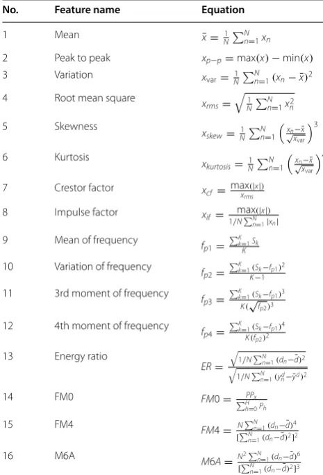
Three types of features are extracted from time domain sig-nal, frequency domain sigsig-nal, and difference sigsig-nal, respec-tively, as given in Table 1. The difference signal is defined as Ref. [4] kept and act as feature weights of the selected
where x is the raw vibration signal, yd is the signal containing the mesh frequencies, their harmonics, and their first-order sidebands. Thus, d is composed of higher-order sidebands and Gaussian noise.
(7) d=x−yd,
Here, x is the original time domain signal; N is the number of samples; Sk is the spectrum of x for k = 1, 2,…, K; K is the number of spectrum lines; y¯d and d¯ are the
mean values of yd and d, respectively; PP
x indicates the maximum peak-to-peak amplitude of signal x; Ph is the amplitude of the hth harmonic; H is the total number of harmonics within the frequency ranges.
In this study, eight features are calculated from time domain signal, four features from frequency domain sig-nal, and four from difference signal. In addition, because the rotating speed is low, the calculated gear mesh fre-quency [36] and its harmonics are concentrated at a low frequency range, and thus, a low-pass digital filter is used to cover the main gear mesh components of the vibra-tion signals, and cut-off frequencies of 650 and 900 Hz are chosen for the low-pass digital filter at 300 and 400 r/min, respectively. Thus, another sixteen features are calculated from the filtered vibration signals, and a total of thirty-two features are obtained within the entire feature set.
3.2 IHFST
To remove both irrelevant and redundant features from the entire feature set, the IHFST method combining DET, Pearson’s correlation analysis, and the ad hoc technique is proposed, as shown in Figure 4. The distance evalua-tion criterion αj of each feature is obtained based on DET, and the entire feature set is then sorted in descending order according to αj. Next, the mean correlation coeffi-cient of the sorted feature set can be computed based on the Pearson’s correlation analysis.
Figure 3 Data segmentation based on sliding window
Table 1 Calculated features
No. Feature name Equation
1 Mean x¯= 1
N
N
n=1xn 2 Peak to peak xp−p=max(x)−min(x)
3 Variation xvar=
1 N
N
n=1(xn− ¯x)2
4 Root mean square x
rms=
1 N
N
n=1x 2 n
5 Skewness x
skew=
1 N
N n=1
xn−¯x
√ xvar
3
6 Kurtosis x
kurtosis=
1
N N
n=1
xn−¯x
√
xvar
4
7 Crestor factor xcf= maxxrms(|x|)
8 Impulse factor xif= 1/NmaxN(|x|) n=1|xn|
9 Mean of frequency f
p1=
K
k=1Sk
K 10 Variation of frequency f
p2=
K
k=1(Sk−fp1)2 K−1
11 3rd moment of frequency f p3=
K
k=1(Sk−fp1)3
K(√fp2)3
12 4th moment of frequency f p4=
K
k=1(Sk−fp1)4
K(fp2)2 13 Energy ratio
ER=
1/NN n=1(dn− ¯d)2
1/NN n=1(ynd−¯yd)2
14 FM0 FM0=HPPx
h=0Ph
15 FM4 FM4= NN
n=1(dn− ¯d)4 [N
n=1(dn− ¯d)2]2
16 M6A M6A= N2N
n=1(dn− ¯d)6
[N
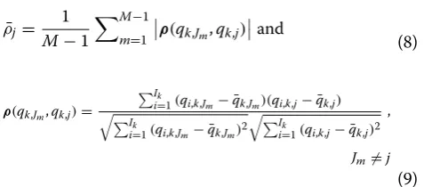
where, ρ¯j is the mean correlation coefficient of the jth fea-ture, M is the ranking index of the jth feature according to αj, Jm is the feature index of the top informative feature for m = 1, 2,…, M − 1, qk,Jm = [q1,k,Jm, q2,k,Jm, . . ., qIk,k,Jm]
and qk,j= [q1,k,j, q2,k,j, . . ., qIk,k,j] are two feature vec-tors, and q¯k,Jm and q¯k,j are the mean values of these two features, respectively. The correlation coefficient ranges from − 1 to + 1, which indicates a high degree of nega-tive or posinega-tive linear correlation between qk,Jm and qk,j.
Finally, the ad hoc technique associated with the mean cor-relation coefficient is applied to reevaluate the distance eval-uation criteria αj, and a feature that is highly correlated with the top informative features will be suppressed or removed. The new distance evaluation criterion βj is obtained, i.e.,
where, θ1 and θ2 are two weighting factors that determine
the relative importance of the informative and the correla-tion terms, respectively. A large θ1 factor emphasizes the
informative term, and a relatively larger θ2 factor weights the
correlation term more heavily, and can thus produce a fea-ture subset with less redundancy [25]. In this paper, when the mean correlation coefficient is higher than 0.7, the feature will be recognized as a severe redundant feature, and will thus be removed. In another situation described herein, the two factors are chosen as θ1 = 1 and θ2 = 0.2.
Hence, a feature subset without irrelevant or redundant features can be selected according to the value of the new distance evaluation criteria βj.
3.3 Normalization and Weighting
Before classification, all features are normalized as follows:
where FEj is the feature to be normalized, mean() is
the mean function, and std() is the standard variance function.
Although the feature subset is selected based on the IHFST, different features in the feature subset have dif-ferent sensitivities during the fault diagnosis process. Thus, to emphasize the importance of sensitive features,
(8)
¯ ρj=
1
M−1
M−1 m=1
ρ(qk,Jm,qk,j) and
(9) ρ(qk,Jm,qk,j)=
Ik
i=1(qi,k,Jm− ¯qk,Jm)(qi,k,j− ¯qk,j)
Ik
i=1(qi,k,Jm− ¯qk,Jm) 2
Ik
i=1(qi,k,j− ¯qk,j)2
,
Jm�=j
(10)
βj=
αj, whenM=1,
θ1αj−θ2ρ¯j, whenM≥2,
(11) nFEj=
FEj−mean(FEj)
std(FEj)
, j=1, 2,. . ., J,
a feature-weighting step is needed to guarantee a more accurate classification result. Supposing there are L fea-tures selected by IHFST, described in Section 3.2, the new distance evaluation criteria βj of these selected features are also kept and act as feature weights of the selected features.
3.4 K‑means Clustering Method
As an unsupervised clustering method, k-means is com-monly used to automatically partition samples into k clusters [31]. The purpose of the k-means clustering method is to assign all N samples into k clusters by mini-mizing the sum of point-to-centroid distances as follows:
where C= {C1,C2,. . .,Ck} indicates k clusters, x is an
N × R feature matrix, R represents the dimensions of the matrix, each row is a single observation or sample, and
µi indicates the cluster centroid of the ith cluster. The
detailed process of the k-means clustering method is given as follows.
Step 1: Initialization
Randomly choose k cluster centroids for all feature samples.
Step 2: Assignation
Assign each sample to the nearest cluster centroid by measuring the distance between the sample and each centroid as follows:
Step 3: Update
Find all samples in each cluster, and determine the new cluster centroid using
where Nit is the sample number of the ith cluster at the tth iteration.
Step 4: Repeat Steps 2 and 3 until the cluster
cen-troid remains unchanged or the function achieves convergence.
4 Experimental System
Figure 5 illustrates the “back-to-back” planetary gear-box experiment setup, which consists of two planetary gearboxes (PGB), two motors, an industrial computer, a control box, and a set of vibration acquisition systems. The test bed is symmetrically arranged, PGB 1 and PGB 2 have the same structure and two motors each, and the
(12)
J=arg min
C
k
i=1
x∈Ci
x�− �µi
,
(13) Cit = {xp :
xp−µti
2
≤ xp−µ
t j 2
∀j, 1≤j≤k}.
(14)
µti+1= 1
Nit
four components are connected using three teeth-shaft couplings.
The design parameters of the PGB are given in Table 2, where the PGB is comprised of an inner sun gear sur-rounded by four planet gears and a standstill ring gear, and the gear ratio of the PGB is 6.25. It should be noted that the simulated faults are located in PGB 1. The two motors are SIEMENS three-phase 15 kW induction motors, where motor 1 is for driving and motor 2 is for loading; in addition, the range of the motor speed is 0–1450 r/min, and the two motors are controlled using an industrial computer through a control box. To meas-ure the vibration signals, five Kistler integrated circuit piezoelectric accelerometers, denoted as #1, #2, #3, #4, and #5, are placed in the test bed. Here, #1 is placed in the motor base, #2 is placed in the housing of the input bearing, #3 is placed in the housing of the planetary gear-box, #4 is placed in the ring gear of the planetary geargear-box, and #5 is placed in the housing of the output bearing, as
illustrated in Figure 5a. An LMS SCADAS system and a computer are used for data acquisition, the sampling fre-quency of which is 20,480 Hz, and the sampling length is 11 s.
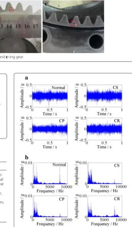
Figure 6a–c illustrate seeded incipient cracks located at the tooth root of the sun gear, planet gear, and ring, respectively. The parameters of the seeded crack are defined as (q0, q1, Wc, αc), as shown in Figure 7. As is well known, it may be more difficult to detect gear faults at low speed because low-frequency characteristics are eas-ily masked by heavy noise [18]. To verify the effective-ness of the proposed method, vibration datasets were collected under two relatively low rotating speeds of 300/400 r/min and four loading conditions of 0, 20, 40, and 60 Nm, as listed in Table 3. Altogether, there were eight vibration datasets collected, each of which includes four types of health conditions: normal, cracked sun gear (CS), cracked planet gear (CP), and cracked ring gear (CR). In addition, the vibration signals of accelerometer #4 mounted on the outer ring gear of PGB 1 were ana-lyzed in this study.
In addition, Figure 8a, b show an example of vibration signals for each health condition in dataset 1 and their spectrum, respectively. It can be observed there are few differences in the raw vibration signals and their spec-trum for the four health conditions: normal, CS, CP, and CR, and it is difficult to distinguish the three types of faults from the normal condition.
5 Results and Discussion
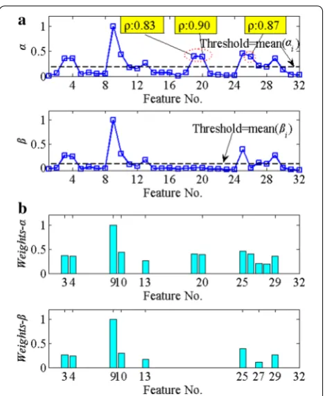
The distance evaluation criteria α and β, and the cor-responding feature weights of dataset 2, are shown in Figure 9a, b, respectively. It can be observed that three features (Nos. 19, 20, and 26) with higher mean cor-relation coefficients in the DET method are suppressed according to the new distance evaluation criteria β. Twelve sensitive features are selected from the entire feature set using the DET method with a given thresh-old, Thr(α) = mean(αj), and eight sensitive features are selected using the IHFST method with a given thresh-old, Thr(β) = mean(βj), where j = 1, 2,…, 32 denotes the feature index. It should be noted that dataset 2 is taken as an example to show the effectiveness of the proposed method, and the other datasets are also analyzed.
In this study, three types of feature selection meth-ods are employed to analyze the same dataset using the proposed method for comparison, which are denoted as Method 1, Method 2, and Method 3. In Method 1, two commonly used features, the root mean square and kur-tosis, are selected from the entire feature set. In Method 2, the dimensions of the entire feature set are directly reduced based on a principle component analysis (PCA) [37] without feature selection. In Method 3, features are Figure 5 “Back‑to‑back” planetary gearbox experiment setup: a
schematic of experimental setup and b photograph of the data acquisition
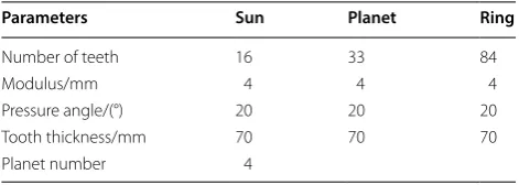
Table 2 Design parameters of planetary gear
Parameters Sun Planet Ring
Number of teeth 16 33 84
Modulus/mm 4 4 4
Pressure angle/(°) 20 20 20
Tooth thickness/mm 70 70 70
selected based on DET. Finally, the proposed method is referred to as Method 4.
The classification performances of these four meth-ods are shown in Figure 10a–d. In addition, it should be noted that, for visualization, the PCA method is implemented based on the clustering results produced through Method 3 and Method 4, and the plots of the first two PCs are shown in Figure 10c, d. Many misclas-sification samples can be found in Figure 10a, b, which are based on Method 1 and Method 2, and the samples have a loose distribution. In Figure 10c, CS and CP can be clearly discriminated, but it is difficult to discrimi-nate the CR from normal conditions, and there are five misclassification samples. In Figure 10d, the four health conditions can be clearly discriminated, and all
four clusters have small within-class distances and large between-class distances.
To compare the classification performance of the four methods, the silhouette value (SV) is adopted in this study. The SV is defined as a measure of how simi-lar a point is to other points in its own cluster compared to points in other clusters, and ranges from − 1 to + 1, where a value close to + 1 indicates a better classification performance [38]. The SV can therefore be obtained:
(15) S(i)= min(b(i, :), 2)−a(i)
max(a(i), min(b(i, :))),
Figure 6 A seeded tooth root crack in a a sun gear, b planet gear, and c ring gear
Figure 7 Parameters of manufactured tooth root crack
Table 3 Working conditions of the experiments Dataset No. Working conditions Crack parameters
1 300 r/min, 0 Nm Each dataset includes four types of health conditions: (1) normal conditions, (2) cracked sun gear (3.5 mm, 1 mm, 3.5 mm, 60°), (3) cracked planet gear (4 mm, 1 mm, 4 mm, 60°), and (4) cracked ring gear (6 mm, 1 mm, 4 mm, 80°)
2 300 r/min, 20 Nm 3 300 r/min, 40 Nm 4 300 r/min, 60 Nm 5 400 r/min, 0 Nm 6 400 r/min, 20 Nm 7 400 r/min, 40 Nm 8 400 r/min, 60 Nm
where a(i) is the average distance from the ith point to other points in its cluster, and b(i, k) is the average dis-tance from the ith point to points in another cluster k. The SV of the classification is obtained based on the aver-age of all S(i).
Table 4 presents the classification results of different datasets based on the four methods, along with their mis-classification error and SV. There are 36 misclassification errors with Method 1, 44 misclassification errors with Method 2, 7 misclassification errors with Method 3, and zero misclassification errors with Method 4. In addition, the SV of Method 4 is greater than that of the other three methods for all datasets.
The improvement of Method 4 over the other three methods is considered to be as follows:
where SVM4 denotes the silhouette values of the
classifi-cation using Method 4, and SVMk denotes these values for the other three methods, for k = 1, 2, and 3.
Figure 11 shows a comparison of the classification per-formance between Method 4 and the other three meth-ods. It can be observed that Method 4 consistently yields a better classification performance than the other three
(16)
Sk =
SVM4−SVMk SVM4
×100%,k=1, 2, 3,
methods for the different datasets. Method 4 achieves a 30.51% to 51.74% improvement over Method 1, 30.92% to 42.43% improvement over Method 2, and 0.89% to 16.45% improvement over Method 3.
As mentioned in Section 3.1, feature extraction is one of the most important steps in the proposed method, and the parameters of the sliding Hanning window have a Figure 9 Comparisons between a distance evaluation criteria α and
β based on DET and IHFST and b the corresponding feature weights of dataset 2
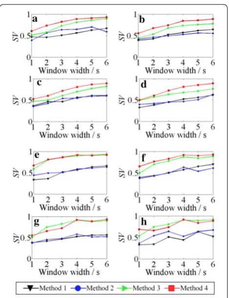
direct influence on the classification performance. There-fore, the effects of the Hanning window width and slid-ing distance on the classification performance of the four methods are illustrated in Figures 12 and 13, respectively.
Figure 12a–h display the effect of the window width on eight datasets, 1 to 8. The window width ranges from 1 to 6 s, and the sliding distance is fixed to 0.5 s. It can be seen that, as the window width increases, the SVs of the four methods show an increasing trend, which may result from too little fault-related information in each segment when the window width is small. In addition, Method 4 shows a higher SV than Method 1 and Method 2 for each dataset, and shows a higher SV than Method 3 for data-sets 1 to 4, and dataset 6.
Figures 13a–h display the effect of the sliding distance on the eight datasets, 1 to 8. The sliding distance ranges from 0.1 to 0.9 s, and the window width is fixed to 4 s. It can be seen that, as the sliding distance increases, the SVs of Method 3 and Method 4 remain nearly unchanged, and the SVs of Method 1 and Method 2 have a small range of fluctuations. In addition, Method 4 shows a
higher SV than Method 1 and Method 2 for each dataset, and a higher SV than Method 3 for most of the datasets.
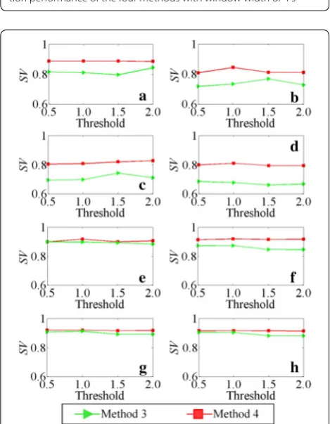
For Method 3 and Method 4, a feature subset is selected from the entire feature set with a given threshold, and it is important to clarify the relationship between the thresh-old and the classification performance. Hence, the effect of the feature selection threshold on the classification performance for Method 3 and Method 4 is also studied, as shown in Figure 14. The thresholds for Method 3 and
Table 4 Classification performance of the four methods Dataset
No. Method 1 Method 2 Method 3 Method 4
Error SV Error SV Error SV Error SV
1 5 0.5618 0 0.6466 0 0.8112 0 0.8871
2 3 0.5702 7 0.5262 5 0.7343 0 0.8435
3 8 0.5610 7 0.5453 0 0.6974 0 0.8073
4 5 0.5213 14 0.4662 2 0.6766 0 0.8098
5 0 0.5688 7 0.5868 0 0.8972 0 0.9172
6 2 0.5754 1 0.6342 0 0.8729 0 0.9180
7 3 0.5224 2 0.5810 0 0.9110 0 0.9192
8 10 0.4417 6 0.5260 0 0.9028 0 0.9153
Figure 11 Comparison of classification performance between Method 4 and the other three methods
Method 4 range from 0.5 × Thr(α) to 2.0 × Thr(α), and from 0.5 × Thr(β) to 2.0 × Thr(β), respectively. It can be seen that, as the threshold increases, the SVs of Method
3 and Method 4 have a small range of fluctuation, and Method 4 shows a higher SV than Method 3 for each dataset.
6 Conclusions
In this paper, an IHFST method combining DET, Pear-son’s correlation analysis, and an ad hoc technique was proposed. A sensitive feature subset without irrelevant or redundant features was selected from the entire feature set based on the proposed IHFST method. The k-means clustering method was further employed to automati-cally partition the vibration data acquired from a plan-etary gearbox with crack faults into several different classifications. To validate the effectiveness of the pro-posed method, three types of feature selection methods were employed to analyze the same dataset using the pro-posed method for comparison. The results indicate that the proposed method can discriminate the four types of health conditions of a planetary gearbox clearly for all the datasets used, and no misclassifications were found. The proposed method achieves a 30.51% to 51.74% improve-ment over Method 1, 30.92% to 42.43% improveimprove-ment over Method 2, and 0.89% to 16.45% improvement over Method 3. In addition, the influence of the sliding Han-ning window and feature selection threshold on the clas-sification performance was investigated, and the proposed method again achieved a better classification performance than the other three methods.
Authors’ contributions
LW carried out the experiment studies and drafted the manuscript. YS carried out the sequence alignment and revision of the manuscript. All authors read and approved the final manuscript.
Authors’ Information
Li‑Ming, Wang born in 1987, is currently a PhD candidate at State Key Labora-tory of Mechanical Transmission, Chongqing University, China. He received his bachelor degree from Chongqing University, China, in 2011. His main research interests include fault diagnosis of rotating machinery and signal processing.
Yi‑Min Shao, born in 1963, is currently a professor at Chongqing University, China. He received his PhD degree from Gunma University, Japan, in 1997. His research interests include mechanical dynamics, signal processing, fault diagnosis of rotating machinery.
Acknowledgements
Supported by National Natural Science Foundation of China (Grant No. 51475053).
Competing interests
The authors declare that they have no competing interests.
Ethics approval and consent to participate
Not applicable.
Publisher’s Note
Springer Nature remains neutral with regard to jurisdictional claims in pub‑ lished maps and institutional affiliations.
Received: 2 January 2017 Accepted: 14 January 2018
Figure 13 Effect of Hanning window sliding distance on classifica‑ tion performance of the four methods with window width of 4 s
References
1. Y C Guo, R G Parker. Analytical determination of mesh phase relations in general compound planetary gears. Mechanism and Machine Theory, 2011, 46(12): 1869–1887.
2. W Smith, L Deshpande, R Randall, et al. Gear diagnostics in a planetary gearbox: a study using internal and external vibration signals. Interna-tional Journal of Condition Monitoring, 2013, 3(2): 36–41.
3. S Sheng, H Link, W LaCava, et al. Wind turbine drivetrain condition monitoring during GRC phase 1 and phase 2 testing. Contract, 2011, 303: 275–300.
4. P Samuel, D J Pines. A review of vibration‑based techniques for helicopter transmission diagnostics. Journal of Sound and Vibration, 2005, 282(1): 475–508.
5. Z G Tian, M J Zuo, S Wu. Crack propagation assessment for spur gears using model‑based analysis and simulation. Journal of Intelligent Manu-facturing, 2012, 23(2): 239–253.
6. J Liu, Y M Shao. Dynamic modeling for rigid rotor bearing systems with a localized defect considering additional deformations at the sharp edges. Journal of Sound and Vibration, 2017, 398: 84–102.
7. W Wang, A K Wong. Autoregressive model‑based gear fault diagnosis. Transactions‑American Society of Mechanical Engineers Journal of Vibration and Acoustics, 2002, 124(2): 172–179.
8. J M Ha, B D Youn, H Oh, et al. Autocorrelation‑based time synchronous averaging for condition monitoring of planetary gearboxes in wind turbines. Mechanical Systems and Signal Processing, 2016, 70: 161–175. 9. H Al‑Bugharbee, I Trendafilova. A fault diagnosis methodology for rolling
element bearings based on advanced signal pretreatment and autore‑ gressive modelling. Journal of Sound and Vibration, 2016, 369: 246–265. 10. Z P Feng, M Liang, Y Zhang, et al. Fault diagnosis for wind turbine plan‑
etary gearboxes via demodulation analysis based on ensemble empirical mode decomposition and energy separation. Renewable Energy, 2012, 47: 112–126.
11. V CMN Leite, J G B da Silva, G F C Veloso, et al. Detection of localized bearing faults in induction machines by spectral kurtosis and envelope analysis of stator current. IEEE Transactions on Industrial Electronics, 2015, 62(3): 1855–1865.
12. B Liang, S D Iwnicki, Y Zhao. Application of power spectrum, cepstrum, higher order spectrum and neural network analyses for induction motor fault diagnosis. Mechanical Systems and Signal Processing, 2013, 39(1): 342–360.
13. C Li, V Sanchez, G Zurita, et al. Rolling element bearing defect detection using the generalized synchrosqueezing transform guided by time–fre‑ quency ridge enhancement. ISA Transactions, 2016, 60: 274–284. 14. B P Tang, W Y Liu, T Song. Wind turbine fault diagnosis based on Morlet
wavelet transformation and Wigner‑Ville distribution. Renewable Energy, 2010, 35(12): 2862–2866.
15. J L Chen, Z P Li, J Pan, et al. Wavelet transform based on inner product in fault diagnosis of rotating machinery: A review. Mechanical Systems and Signal Processing, 2016, 70: 1–35.
16. Z W Gao, C Cecati, S X Ding. A survey of fault diagnosis and fault‑tolerant techniques—Part I: Fault diagnosis with model‑based and signal‑based approaches. IEEE Transactions on Industrial Electronics, 2015, 62(6): 3757–3767.
17. V Muralidharan, V Sugumaran. Rough set based rule learning and fuzzy classification of wavelet features for fault diagnosis of monoblock cen‑ trifugal pump. Measurement, 2013, 46(9): 3057–3063.
18. Y G Lei, J Lin, M J Zuo, et al. Condition monitoring and fault diagnosis of planetary gearboxes: A review. Measurement, 2014, 48: 292–305. 19. Y G Lei, M J Zuo. Gear crack level identification based on weighted K
nearest neighbor classification algorithm. Mechanical Systems and Signal Processing, 2009, 23(5): 1535–1547.
20. M Kang, M R Islam, J Kim, et al. A hybrid feature selection scheme for reducing diagnostic performance deterioration caused by outliers in data‑driven diagnostics. IEEE Transactions on Industrial Electronics, 2016, 63(5): 3299–3310.
21. S Theodoridis, K Koutroumbas. Pattern Recognition, Fourth Edition. Burling‑ ton, MA: Academic Press, 2008.
22. H C Peng, F H Long, C Ding. Feature selection based on mutual informa‑ tion criteria of max‑dependency, max‑relevance, and min‑redundancy. IEEE Transactions on Pattern Analysis and Machine Intelligence, 2005, 27(8): 1226–1238.
23. J Yang, V Honavar. Feature subset selection using a genetic algorithm. IEEE Intelligent Systems and Their Applications, 1998, 13(2): 44–49. 24. B Li, P L Zhang, H Tian, et al. A new feature extraction and selection
scheme for hybrid fault diagnosis of gearbox. Expert Systems with Applica-tions, 2011, 38(8): 10000–10009.
25. Z L Liu, J Qu, M J Zuo, et al. Fault level diagnosis for planetary gearboxes using hybrid kernel feature selection and kernel Fisher discriminant analysis. The International Journal of Advanced Manufacturing Technology, 2013, 67(5‑8): 1217–1230.
26. Y G Lei, Z J He, Y Y Zi, et al. New clustering algorithm‑based fault diag‑ nosis using compensation distance evaluation technique. Mechanical Systems and Signal Processing, 2008, 22(2): 419–435.
27. Z J Shen, X F Chen, X L Zhang, et al. A novel intelligent gear fault diagno‑ sis model based on EMD and multi‑class TSVM. Measurement, 2012, 45(1): 30–40.
28. B S Yang, K J Kim. Application of Dempster–Shafer theory in fault diagno‑ sis of induction motors using vibration and current signals. Mechanical Systems and Signal Processing, 2006, 20(2): 403–420.
29. Q Hu, Z J He, Z S Zhang, et al. Fault diagnosis of rotating machinery based on improved wavelet package transform and SVMs ensemble. Mechani-cal Systems and Signal Processing, 2007, 21(2): 688–705.
30. A Widodo, B S Yang. Support vector machine in machine condition moni‑ toring and fault diagnosis. Mechanical Systems and Signal Processing, 2007, 21(6): 2560–2574.
31. M Yuwono, Y Guo, J Wall, et al. Unsupervised feature selection using swarm intelligence and consensus clustering for automatic fault detec‑ tion and diagnosis in heating ventilation and air conditioning systems. Applied Soft Computing, 2015, 34: 402–425.
32. C T Yiakopoulos, K C Gryllias, I A Antoniadis. Rolling element bearing fault detection in industrial environments based on a K‑means clustering approach. Expert Systems with Applications, 2011, 38(3): 2888–2911. 33. G F Wang, C Liu, Y H Cui. Clustering diagnosis of rolling element bearing
fault based on integrated autoregressive/autoregressive conditional heteroscedasticity model. Journal of Sound and Vibration, 2012, 331(19): 4379–4387.
34. M E Celebi, H A Kingravi, P A Vela. A comparative study of efficient initiali‑ zation methods for the k‑means clustering algorithm. Expert Systems with Applications, 2013, 40(1): 200–210.
35. J Barros, R I Diego. On the use of the Hanning window for harmonic analysis in the standard framework. IEEE Transactions on Power Delivery, 2006, 21(1): 538–539.
36. Z P Feng Z, M J Zuo. Vibration signal models for fault diagnosis of plane‑ tary gearboxes. Journal of Sound and Vibration, 2012, 331(22): 4919–4939. 37. J Harmouche, C Delpha, D Diallo. Incipient fault detection and diagnosis based on Kullback–Leibler divergence using principal component analy‑ sis: Part II. Signal Processing, 2015, 109: 334–344.