O R I G I N A L R E S E A R C H
Open Access
Bayesian estimation of the reliability
characteristic of Shanker distribution
Tahani A. Abushal
Correspondence: [email protected] Department of Mathematics, Faculty of Science, Umm AL-Qura University, Makkah, Saudi Arabia
Abstract
In this study, we discussed the Bayesian property of unknown parameter and reliability characteristic of the Shanker distribution. The maximum likelihood estimate is
calculated. The approximate confidence interval of the unknown parameter is
constructed based on the asymptotic normality of maximum likelihood estimator. Two bootstrap confidence intervals for the unknown parameter are also computed. Bayesian estimates of parameter and reliability characteristic against squared error loss function are obtained. Lindley’s approximation and Metropolis-Hastings algorithm are applied to obtain the Bayes estimates. In consequence, we also construct the highest posterior density intervals. A numerical comparison is also made to compare different methods through a Monte Carlo simulation study. Finally, two real data sets are also analyzed using the proposed methods.
Keywords: Shanker distribution, Maximum likelihood estimate, Bootstrap technique,
Metropolis-hastings algorithm
2010 Mathematics Subject Classification: 62F10
Introduction
In the literature, a continuous one-parameter distribution named the “Shanker distribu-tion” has its origin in the papers by Shanker [1]. Shanker distribution has been found useful for modeling lifetime data from engineering and medical science. The author studied its mathematical and statistical properties. He discussed its shape, moments, skewness, kurtosis, and also its reliability characteristics. The author also obtained the Bayesian estimation of the unknown parameter and applications for modeling lifetime data from engineering and biomedical science.
The Shanker distribution with parameterθ has the probability density function (PDF) and cumulative distribution function (CDF), respectively,
fX(x)= θ
2
(θ2+1)(θ+x)e
−θx, x>0, θ >0, (1)
FX(x)=1−(θ
2+θx+1)
(θ2+1) e
−θx, x>0. (2)
This distribution is the mixture of the exponential (θ)and gamma (2,θ) with their mixing proportions θ2θ+12 andθ21+1respectively.
Then, the corresponding reliability function, hazard function, and mean residual life function ofXare given, respectively, by
R(t)=
θ2+θt+1
(θ2+1) e
−θt, t>0, (3)
h(t)= θ 2(θ+t)
θ2+θt+1, t>0. (4)
m(t)=
θ2+θt+2
θθ2+θt+1, t>0. (5) In recent years, several researchers have investigated the inference problems for Shanker distribution. In the literature, Shanker distribution has its origin in the papers by Shanker [1]. He discussed statistical properties of Shanker distribution. In this paper, the author discussed some inferential issues also. Three real-life data sets are provided to illustrate its exibility and potentiality over the lindley and exponential distribution. Shanker and Fesshay [2] studied the modeling of lifetime data using one-parameter Akash, Shanker, Lindley, and exponential distributions.
Recently, many authors consider Bayesian estimation for univariate distributions. Ras-togi and Merovci [3] detailed the study about the Bayesian estimation for parameters and reliability characteristics of the Weibull Rayleigh distribution. Chandrakant et al. [4] dis-cussed various inference properties of a Weibull inverse exponential distribution. The authors estimated the unknown parameters using classical and Bayesian techniques. Two real data sets are analyzed in support of the proposed estimation.
We obtain the different classical and Bayesian point estimators of unknown parame-ter using maximum likelihood and Bayesian methods of estimation. The Bayes estimates of unknown parameter are derived under the squared error loss function. We obtain the interval estimation. The approximate and two bootstrap confidence intervals (CIs) are derived. The highest posterior density (HPD) interval is considered as well. These point and interval estimators are treated as an important problem in many practical applications as well as financial, industrial, agricultural, and reliability experiments.
The layout of the paper is as follows: In “The maximum likelihood estimation” section, the maximum likelihood estimate(MLE) of the unknown parameter is obtained. The approximate and two bootstrap (CIs) are derived in the “Confidence intervals” section. In “The Bayesian estimation” section, the Bayes estimates relative to square error loss func-tion and HPD interval are considered. The Monte Carlo simulafunc-tion results are presented in the “Numerical comparison” section. The “Data analysis” section provided the illus-tration of the proposed procedure by using a real-life data. Eventually, the conclusion is inserted in the “Conclusions” section.
The maximum likelihood estimation
Suppose thatX1,X2,. . .,Xn is a random sample ofn-independent units obtained from a Shanker distribution as defined in (1). The likelihood ofθ for the model (1) can be described as
L(θ)∝ θ 2ne−θs
(θ2+1)n n
i=1
(θ+xi) (6)
wheres=ni=1xi. The logarithm of the likelihood (6) is
logL(θ)∝2nlogθ−nlogθ2+1−θs+ n
i=1
Making the differentiation of Eq. (7) with respect toθ and then equating them to zero, we have, respectively,
dlogL
dθ =
2n θ −
2nθ θ2+1−s+
n
i=1 1
(θ+xi) =0. (8)
The MLEθˆ of θ is a solution of Eq. (8). We observe that θˆ can not be obtained in closed form and have to solve Eq. (8) numerically to obtain the desired estimate. So, some numerical technique, for instance, the Newton- Raphson and Broydan method, may be used. We used the package “nleqslv" in (software) R to find the solution of the unknown parameterθ.
Note that (8) can be written in the form:
θ =h(θ) (9)
where
h(θ)=2n
2nθ θ2+1 +s−
n
i=1 1 (θ+xi)
−1
We design a simple iterative scheme to solve the above Eq. (9) forθ. We can start with an initial guess ofθ, sayθ(0), then findθ(1) =h(θ(0))and, proceeding in this way, obtain θ(k) = hθ(k−1). Stop the iterative procedure, when θ(k)−θ(k−1) < η, whereηsome pre-assigned tolerance limit.
Finally, using the invariance property of the MLE, the MLEs ofR(t),h(t), andm(t) , respectively, defined asRˆ(t),hˆ(t), andmˆ(t), are obtained as
ˆ
R(t)= (θˆ
2+ ˆθt+1)
(θˆ2+1) e
− ˆθt, hˆ(t)= θˆ2(θˆ+t)
(θˆ2+ ˆθt+1), and m(t)=
(θˆ2+ ˆθt+2)
ˆ
θ(θˆ2+ ˆθt+1) t>0. In next section, we obtain asymptotic intervals ofθusing asymptotic normality property of MLEs.
Confidence intervals
Approximate CI
The asymptotic variance of θˆ for Shanker distribution is given byVar(θ)ˆ =[IX(θ)ˆ ]−1
whereI(θ)ˆ is the observed Fisher’s information which is given byI(θ)ˆ = −d2dlogθ2L
θ= ˆθ .
Since the Shanker distribution belongs to one-parameter exponential family of distribu-tions, therefore, the sampling distribution of √(θ−θ)ˆ
Var(θ)ˆ can be approximated by a standard normal distribution. The symmetric 100(1−ξ)% approximate CI for the parameterθ is
then obtained byθˆ±zξ 2
Var(θ)ˆ , where 0< ξ < 1 andzξ
2 denotes the upper ξ 2th per-centile of the standard normal distribution. Using the simulation, we can estimate the coverage probability
P ⎡ ⎢ ⎣ (θˆ−θ)
Var(θ)ˆ ≤zξ
2
⎤ ⎥ ⎦.
Bootstrap CIs
We propose to use CIs based on the parametric bootstrap methods. It is known that CIs with the asymptotic results do not implement very well for small samples. There are three types of resampling plans: non-parametric, semi-parametric, and parametric. The bootstrap techniques depend on these three resampling plans, see Efron [5]. We used the parameteric bootstrap methods where the parametric model for the data is known fx; . up to the unknown parameter θ, so that the bootstrap data are sampled from
f
x;θˆ
, whereθˆis the MLE from the original data. Many studies dealt with percentile bootstrap method (Boot-p) based on the idea of Efron and Tibshirani [6] and bootstrap-t method (Boot-t) based on the idea of Hall [7] and Hall [8], such as Kundu and Joarder [9] among others. Kundu and Joarder [9] proposed two parametric bootstrap confidence intervals for the unknown parameter, say θ. The following procedures are followed to obtain bootstrap samples for the two methods:
The following steps are required to construct CI using Boot-p method:
1. Draw sampleX1,X2,. . .,Xnfrom (1) and calculate the estimateθˆ.
2. Next, draw a bootstrap sampleX1∗,X2∗,. . .,Xn∗usingθˆ. Derive the updated
bootstrap estimate ofθ, sayθˆ∗, using this sample.
3. Repeat Step [2]B times.
4. LetF(x)=P(θˆ∗≤x)be the cumulative distribution function ofθˆ∗. Then, define
ˆ
θBoot−p(x)=F−1(x)for a givenx. The approximate100(1−ξ)%CI forθis given by
ˆ θBoot−p
ξ
2
, θBootˆ −p
1−ξ2,
and the following steps are required to construct CI using Boot-t method:
1. Draw sampleX1,X2,. . .,Xnfrom (1) and obtain the estimateθˆ.
2. Next, draw a bootstrap sampleX1∗,X2∗,. . .,Xn∗usingθˆ. Then, derive the estimates
ˆ
θ∗andVˆ(θˆ∗).
3. Obtain theT∗statistic defined as
T∗= √θˆ∗− ˆθ ˆ
V(θˆ∗).
4. Repeat Step 2 B times.
5. LetF(x)=P(T∗≤x)be the cumulative distribution function ofT∗. Define
ˆ
θBoot−t(x)= ˆθ+
ˆ
V(θˆ∗)F−1(x)for a givenx. The approximate100(1−ξ)%CI
forθis given by
ˆ θBoot−t
ξ
2
, θˆBoot−t
1− ξ2.
The Bayes estimators of unknown parameter and reliability characteristics are obtained in the next section.
The Bayesian estimation
The Bayesian inference procedures have been developed under the usual squared error loss function (quadratic loss), which is symmetrical, and associates equal importance to the losses due to overestimation and underestimation of equal magnitude. One may refer to paper by Canfield [10] for detail exposition in this direction. The mathematical form of squared loss function may simply be expressed as:
Squared error loss : Ls(υ,η) = (η−υ)2.
π(θ)∝ θa−1e−bθ θ >0, a>0,b>0. (10)
After a simple calculation, the posterior distribution ofθ is obtained as
π(θ|x)∝ θ
2n+a−1e−θ (b+s)
(θ2+1)n n
i=1
(θ+xi), (11)
where x=(x1,x2,. . .,xn).
Now, the corresponding Bayes estimate ofθagainst the loss functionLsis obtained as
˜
θs=E[θ|x ]= 1 k
∞
0
θ2n+a (θ2+1)ne−θ (
b+s) n
i=1
(θ+xi)dθ,
k=
∞
0
θ2n+a−1 (θ2+1)ne
−θ (b+s)n
i=1
(θ+xi)dθ.
Next, the Bayes estimates of R(t),h(t) and m(t) with respect to square error loss function can be written, as
˜
Rs(t)= 1 k
∞
0
θ2n+a−1(θ2+θt+1)
(θ2+1)(n+1) e−θ (b+s+t)
n
i=1
(θ+xi)dθ,
˜
hs(t)= 1 k
∞
0
θ2n+a+1(θ+t) (θ2+θt+1)(θ2+1)ne
−θ (b+s) n
i=1
(θ+xi)dθ,
˜
ms(t)= 1 k
∞
0
θ2n+a−2(θ2+θt+2)
(θ2+θt+1) (θ2+1)ne
−θ (b+s) n
i=1
(θ+xi)dθ,
It is clear that all the above Bayes estimators do not have simple closed forms. There-fore, in next sections, we employ two popular approximation procedures to calculate the approximate Bayes estimates of the parameter and reliability characteristic.
Lindley’s approximation
In the previous subsection, we obtained the Bayes estimates ofθunder squared error loss function. These estimates are of the form of the ratio of the two integrals. Lindley [11] developed a procedure to approximate the ratio of the two integrals. In this subsection, using this technique, we obtain the approximate Bayes estimates ofθunder the stated loss functions. For illustration, consider the ratio of integral I(x), where
I(x)=
θu(θ)el(θ)+ρ(θ)dθ θ el(θ)+ρ(θ)dθ
, (12)
whereu(θ)is function ofθ only andl(θ)is the log-likelihood andρ(θ)=logπ(θ). Letθˆ denote the MLE ofθ. Applying Lindley’s approximation procedure,I(x)can be written as
I(x)=u(θ)ˆ +0.5uˆθθ+2uˆθρˆθσˆθθ+ ˆuθσˆθθ2 ˆlθθθ
,
whereuθθdenotes the second derivative of the functionu(θ)with respect toθ, anduˆθθ represents the same expression evaluated atθ = ˆθ. All other quantities appearing in the above expression ofI(x)are interpreted as follows
ˆ
lθθ0 = ∂ 2l
∂θ2
θ= ˆθ = − 2n
ˆ θ2 −
2n(θ2−1) (θ2+1)2 −
n
i=1 1
(θˆ+xi)2, σˆθθ = − 1
ˆlθθ ,
ˆlθθθ = ∂3l ∂θ3
θ= ˆθ = 4n
ˆ θ3 +
4nθ (θ2−3) (θ2+1)3 +
n
i=1 2
(θˆ+xi)3, ρˆθ=
(a−1)
Now, to obtain the Bayes estimate ofθ under the loss functionLs, we have
u(θ)=θ, uθ =1, uθθ =0, θs˜ = ˆθ+0.5uˆθθ+2uˆθρˆθ σˆθθ+ ˆuθ σˆθθ2 ˆlθθθ
.
In a similar manner, we can derive the Bayes estimates ofR(t),h(t), and m(t) with respect to the square error loss functions.
In the next subsection, we use the Metropolis-Hastings (MH) algorithm and compute some more estimates of unknown parameter. One may refer to Metropolis et al. [12] and Hastings [13] for various applications of this method.
Metropolis-Hastings algorithm
We generate samples from the given posterior distribution using the normal as proposal distribution forθ. We need the following procedure to generate posterior samples using the proposed algorithm.
Step 1:Choose an initial guess ofθand call itθ0.
Step 2:Generateθusing the proposalNθn−1,σ2distribution.
Step 3:Computeh= π(θπ(θ|x)
n−1|x).
Step 4:Then, generate a sampleufrom the uniformU(0, 1)distribution.
Step 5:Ifu≤h, then set
θn→θ; otherwise θn→θn−1.
Step 6:Repeat steps (2–5)Qtimes and collect adequate number of replicates.
In order to avoid dependence of the sample on the initial values, the first few samples are discarded, and to minimize the correlation between subsequent samples, lagging is used. Then, the resulting sample is approximately independent. In this way, we are able to generate sample from the posterior distribution ofθ. Suppose thatQdenotes the total number of generated sample andQ0denotes the initial burn-in sample.
Finally, we observe that the associated Bayes estimate of θ under square error loss function is given by
ˆ θMH,s=
1 Q−Q0
Q
i=Q0+1 θi.
Finally, we observe that the associated Bayes estimate ofR(t)under square error loss function is given by
ˆ
R(t)s= 1 Q−Q0
Q
i=Q0+1
θ2
i +θit+1
θ2
i +1
e−θit.
In a similar manner, we can derive the Bayes estimates ofh(t)andm(t)with respect to the square error loss functions.
It should be noticed that the 100(1−ξ)% HPD interval for the unknown parameterθ can easily be constructed using the MH samples. The idea was developed by Chen and Shao [14]. First, arrange the sampleθ1,θ2, ...,θQin increasing order. Then, the 100(1−ξ)% credible interval forθ is obtained as(θ1,θ (1−ξ)Q+1),...,(θQξ,θQ), where zdenotes the greatest integer less than or equal toz. Among all such credible intervals, the shortest one is the HPD interval.
Numerical comparison
Table
1
Average
and
MSEs
values
of
all
estimates
of
θ
for
different
choices
of
n
˜θLI ˜θMH
ˆθ
N
IPI
PN
IP
IP
n
EV
MSE
EV
M
SE
EV
MSE
EV
M
SE
EV
MSE
30
0.507092
0.003855
0.504531
0.003701
0.504824
0.003325
0.503879
0.003649
0.504991
0.003356
50
0.50346
0.002263
0.502597
0.002241
0.502167
0.002054
0.502692
0.002261
0.502418
0.002059
70
0.502668
0.001582
0.502054
0.001572
0.50177
0.001490
0.502241
0.001562
0.502068
0.001499
90
0.502061
0.001237
0.501586
0.001238
0.501634
0.001164
0.501864
0.001235
0.501966
0.001176
110
0.501928
0.001014
0.50154
0.001007
0.501377
0.000962
0.501718
0.001010
0.501465
Table 2 Average and MSEs values of all estimates of R ( t ) for different choices of n and T T =1 .5 T =4
˜R(LI
t
)
˜RMH
(
t
)
˜R(LI
t
)
˜RMH
(
t
)
n
ˆR(t
) NIP IP N IP IP
ˆR(t
Table 3 Average and MSEs values of all estimates of h ( t ) for different choices of n and T T =1 T =5
˜h(LI
t
)
˜hMH
(
t
)
˜h(LI
t
)
˜hMH
(
t
)
n
ˆh(t
) NIP IP N IP IP
ˆh(t
Table
5
Estimated
coverage
probabilities
(in%)
and
average
lengths
of
interval
estimates
of
θ
for
different
choices
of
n
Coverage
probability
Average
length
n
Boot-p
Boot-t
Approx
HPD
Boot-p
Boot-t
Approx
HPD
NIP
IP
N
IP
IP
30
0.956
0.946
0.95
0.9155
0.9243
0.242026
0.237732
0.238356
0.207345
0.200522
50
0.95
0.949
0.9489
0.9256
0.9323
0.185804
0.18376
0.18373
0.170139
0.166896
70
0.95
0.951
0.9502
0.9347
0.9374
0.155684
0.155238
0.155037
0.146884
0.130134
90
0.952
0.94
0.9507
0.9339
0.9351
0.13759
0.136508
0.136568
0.131053
0.129815
110
0.961
0.948
0.95
0.9375
0.9388
0.123808
0.123203
0.123493
0.119556
simulation study was conducted and the results are presented in this section. For the sim-ulation study, we tookθ = 0.5,n = 30, 50, 70, 90, 110. The main idea to take different combinations of nis to see how the MLE and Bayes estimates perform for them. The informative and non-informative prior were used to obtain the Bayes estimates and HPD intervals. The hyper-parameters were taken as follows:a=4,b=8 for informative prior anda=0,b =0 for non-informative prior. They were chosen such that the expectation of prior match with the true parameter value. To obtain the Bayes estimates and HPD intervals using MH algorithm, we setQ=10000 replications andQ0= 2000 as the initial burn-in sample. In all cases, Bayes estimates are against square error loss function. Under these settings, the average estimates and the estimated mean squared errors (MSEs) of different estimates based on the 10000 simulated complete samples from the Shanker dis-tribution are listed in Tables1,2,3, and4. Also, for comparison purposes, using simulated samples, the coverage probabilities and average lengths of various CIs and HPD intervals based on 95% of the true coverage probability were computed. To obtain the bootstrap CIs, we setB=10000 replications. The average lengths and the corresponding coverage probabilities are reported in Table5.
All the computations were conducted in R software (R i386 3.2.2), and R codes can be obtained from the author upon request. Some of the points are quite clear from the simulation study. Based on tabulated the average estimates, the estimated MSE, cover-age probability, and avercover-age length values following the conclusions can be drawn from Tables1,2,3,4, and5.
1. It is observed that the average estimates of the MLE and Bayes estimates are all
close to the true parameter for different combinations ofn. Also, the performance
of the MLE and Bayes estimates of the unknown parameter is quite satisfactory, in terms of their MSEs. We found that Bayes estimators have smaller MSE values
than the MLE ofθ.
2. The performance of the Lindley estimates is very similar to that of the
corresponding Bayes estimates using the MH algorithm.
3. As expected, the MSE values of all estimates decrease as the sample sizen grows.
4. It is observed that coverage probabilities obtained by approximate CI, Boot-p, and
Boot-t CIs are better than HPD interval and they are close to the nominal level. But HPD interval provides a good balance between the coverage probabilities as well as average lengths. Therefore, in general, we would recommend to use the HPD interval. If one wants to guarantee that the coverage probability is close to the nominal level and the length of HPD interval is not the major concern, then approximate CI and Boot-t CI are proposed in most cases.
5. From the comparison of Boot-p and Boot-t CIs, it is observed that the performance
of Boot-t CI is marginally better than Boot-p CI in terms of average lengths and coverage probabilities.
Data analysis
For illustrative purposes, we have analyzed two real data sets which have been recently considered by Ghitany et al. [15]. They fitted these real data sets to the Shanker
Table 6Point and interval estimates ofθfrom data set 1
ˆ
θ θ˜LI θ˜MH Boot-p Boot-t Approx HPD
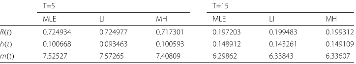
Table 7Point estimates ofR(t),h(t)andm(t)for different choices ofTfrom data set 1
T=5 T=15
MLE LI MH MLE LI MH
R(t) 0.724934 0.724977 0.717301 0.197203 0.199483 0.199312
h(t) 0.100668 0.093463 0.100593 0.148912 0.143261 0.149109
m(t) 7.52527 7.57265 7.40809 6.29862 6.33843 6.33607
distribution and found that the Shanker distribution fits both real data sets reasonably good. They also obtained useful inference for the prescribed model.
Data set 1:The first data-set represents the waiting times (in minutes) before service of 100 bank customers and was examined and analyzed by Ghitany et al. (2008) for fitting the Lindley distribution. The data are as follows:
0.8, 0.8, 1.3, 1.5, 1.8, 1.9, 1.9, 2.1, 2.6, 2.7, 2.9, 3.1, 3.2, 3.3, 3.5, 3.6, 4.0, 4.1, 4.2, 4.2, 4.3, 4.3, 4.4, 4.4, 4.6, 4.7, 4.7, 4.8, 4.9, 4.9, 5.0, 5.3, 5.5, 5.7, 5.7, 6.1, 6.2, 6.2, 6.2, 6.3, 6.7, 6.9, 7.1, 7.1, 7.1, 7.1, 7.4, 7.6, 7.7, 8.0, 8.2, 8.6, 8.6, 8.6, 8.8, 8.8, 8.9, 8.9, 9.5, 9.6, 9.7, 9.8, 10.7, 10.9, 11.0, 11.0, 11.1, 11.2, 11.2, 11.5, 11.9, 12.4, 12.5, 12.9, 13.0, 13.1, 13.3, 13.6, 13.7, 13.9, 14.1, 15.4, 15.4, 17.3, 17.3, 18.1, 18.2, 18.4, 18.9, 19.0, 19.9, 20.6, 21.3, 21.4, 21.9, 23.0, 27.0, 31.6, 33.1, 38.5
Based on the original data, the MLEs of unknown parameter θ were evaluated from Eq. (8). We also computed different Bayes estimates under square error loss function using Lindley’s approximation and MH algorithm. Since we did not have any prior information onaandb, we assumed the non-informative prior, i.e., a=b=0. The MLEs and all Bayes estimates of unknown parameterθare displayed in Table6, and also, we constructed the approximate CI, Boot CIs, and HPD interval. From Table6, it is observed that all the esti-mates are close to each other. The HPD interval performs better among all the intervals in respect of length. The MLEs and Bayes estimates of reliability characteristics are derived in Table7.
Data set 2:This data set is the strength data of glass of the aircraft window reported by Fuller et al. [16]. The data are as follows
18.83, 20.80, 21.65, 23.03, 23.23, 24.05, 24.32, 25.50, 25.52, 25.8, 26.69, 26.77, 26.78, 27.05, 27.67, 29.90, 31.11, 33.20, 33.73, 33.76, 33.89, 34.76, 35.75, 35.91, 36.98, 37.08, 37.09, 39.58, 44.05, 45.29, 45.38.
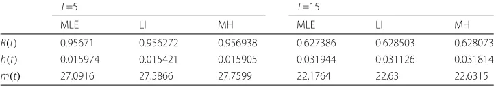
Table8shows the MLEs and Bayes estimates of the unknown parameterθ. The 95% CIs, Boot CIs, and HPD intervals forθ are also presented in Table8. All the Bayes estimates and HPD intervals were evaluated against non-informative prior distribution. Similar to the obtained result from data set 1, we observe that the MLE and Bayes procedures have similar values forθ. Also, HPD intervals have shortest lengths among all the interval estimates. In Table9, the classical and Bayes estimation of reliability characteristics are calculated.
Table 8Point and interval estimates ofθfrom data set 2
ˆ
θ θ˜LI θ˜MH Boot-p Boot-t Approx HPD
Table 9Point estimates ofR(t),h(t), andm(t)for different choices ofTfrom data set 2
T=5 T=15
MLE LI MH MLE LI MH
R(t) 0.95671 0.956272 0.956938 0.627386 0.628503 0.628073
h(t) 0.015974 0.015421 0.015905 0.031944 0.031126 0.031814
m(t) 27.0916 27.5866 27.7599 22.1764 22.63 22.6315
Conclusions
In this paper, we have discussed the classical and Bayesian inferential of unknown param-eter and reliability characteristics of the Shanker distribution. We have provided the MLE and Bayes estimates and the corresponding CIs and HPD interval. A numerical simula-tion has been conducted to compare the performance of different methods, and results of a simulation study have been reported comprehensively in this paper. The method can be extended for progressively type-I hybrid censoring scheme and other censoring schemes also. We believe that more work is needed along these directions.
Abbreviations
BE: Bayes estimate; CDF: Cumulative distribution function; CIs: Confidence intervals; HPD: Highest posterior density; ML: Maximum likelihood; MLE: ML estimate; MSE: Mean squared error; PDF: Probability density function
Acknowledgments Not applicable.
Funding
There are no sources of funding for the research.
Availability of data and materials It is not applicable in my paper.
Author’s contributions
The author read and approved the final manuscript.
Competing interests
The author declares that he/she has no competing interests.
Publisher’s Note
Springer Nature remains neutral with regard to jurisdictional claims in published maps and institutional affiliations.
Received: 3 July 2018 Accepted: 27 December 2018
References
1. Shanker, R.: Shanker distribution and its applications. Int. J. Stat. Appl.5(6), 338–348 (2015)
2. Shanker, R., Fesshay, H.: On modeling of lifetime data using one parameter Akash, Shanker, Lindley and exponential distributions. Biom. Biostat. Int. J.3(6), 00084 (2016)
3. Rastogi, M. K., Merovci, F.: Bayesian estimation for parameters and reliability characteristic of the Weibull Rayleigh distribution. J. King Saud Univ. Sci.30(4), 472–478 (2018)
4. Chandrakant Rastogi, M. K., Tripathi, Y. M.: On a Weibull-Inverse Exponential Distribution. Ann. Data. Sci.5(2), 209–234 (2018)
5. Efron, B.: The jackknife, the bootstrap, and other resampling plans. CBMS-NSF Regional Conference Series in Applied Mathematics. Philadelphia. Society for Industrial and Applied Mathematics (SIAM) (1982)
6. Efron, B., Tibshirani, R.: Bootstrap methods for standard errors, confidence intervals, and other measures of statistical accuracy. Stat. Sci.1, 54–77 (1986)
7. Hall, P.: Theoretical comparison of bootstrap confidence intervals. Ann. Stat.16, 927–953 (1988) 8. Hall, P.: The bootstrap and edgeworth expansion. Springer-Verlag, New York (1992)
9. Kundu, D., Joarder, A.: Analysis of type-II progressively hybrid censored data. Comput. Stat. Data Anal.50, 2509–2528 (2006)
10. Canfield, R. V.: A Bayesian approach to reliability estimation using a loss function. IEEE Trans. Reliab.19(1), 13–16 (1970)
12. Metropolis, N., Rosenbluth, A. W., Rosenbluth, M. N., Teller, A. H., Teller, E.: Equations of state calculations by fast computing machines. J. Chem. Phys.21, 1087–1092 (1953)
13. Hastings, W. K.: Monte Carlo sampling methods using Markov chains and their applications. Biometrika.57, 97–109 (1970)
14. Chen, M. H., Shao, Q. M.: Monte Carlo estimation of Bayesian credible and HPD intervals. J. Comput. Graph. Stat.8, 69–92 (1999)
15. Ghitany, M. E., Atieh, B., Nadarajah, S.: Lidley distribution and its application. Math. Comput. Simul.78, 493–506 (2008) 16. Fuller, E. J., Frieman, S., Quinn, J., Quinn, G., Carter, W.: Fracture mechanics approach to the design of glass aircraft
windows: A case study. SPIE Proc.2286, 419–430 (1994)