Adv. Radio Sci., 13, 19–29, 2015 www.adv-radio-sci.net/13/19/2015/ doi:10.5194/ars-13-19-2015
© Author(s) 2015. CC Attribution 3.0 License.
Efficient determination of the left-eigenvectors for
the Method of Lines
S. F. Helfert
FernUniversität in Hagen, Hagen, Germany
Correspondence to: S. Helfert ([email protected])
Received: 15 December 2014 – Revised: 8 April 2015 – Accepted: 21 May 2015 – Published: 3 November 2015
Abstract. The efficient determination of left eigenvectors in the method of lines (MoL) is described in this paper. The electromagnetic fields are expanded into eigenmodes and the eigenmodes are determined from an explicit matrix eigenvec-tor problem. To study complicated structures with a moderate numerical effort, the analysis is done with a reduced set of these eigenmodes. The enforcements of the continuity of the transverse electric and magnetic fields at interfaces leads to expressions with rectangular matrices. Now left eigenvectors can be considered as inverse of these rectangular matrices. Until now, the left eigenvectors were determined from a sec-ond explicit eigenvalue problem. Here, it is shown how they can be determined with simple matrix products from previ-ously determined right eigenvectors. This is done by utiliz-ing the relation between the transverse electric and magnetic fields. The derived formulas hold for structures with Dirich-let, Neumann or periodic boundary conditions and the ma-terials may be lossy. Open structures are modeled with per-fectly matched layers (PML). To verify the expressions, var-ious devices that contain such PMLs and lossy metals were studied. In all cases, error measures show that the algorithm derived in this paper works very well.
1 Introduction
Complicated waveguide structures can be analyzed analyti-cally only in exceptional cases. Therefore, usually numerical methods are used for this purpose. There are various possibil-ities to classify these methods, e.g. according to their analyt-ical/numerical part. In the well known finite difference time domain method (FDTD, see e.g. Taflove, 1995) all deriva-tives that occur in Maxwell’s equations are discretized with finite differences. Since all points in space and time are
dis-cretized, the simulation of complicated structures can be nu-merically demanding.
On the other side there are eigenmode algorithms (see e.g. Sudbø, 1993; Sztefka, 1992). Here, analytic expressions are used at least in the direction of wave propagation. Con-tinuously varying structures are typically modeled with a stair-case approximation. Besides, usually the analytic ex-pressions exist of infinite series, which must be truncated in practical applications. Therefore, in spite of its analytic formulation, approximations are also introduced in case of eigenmode methods. There exist various ways in computing the eigenmodes and it is not always easy to determine all important ones with analytic expressions in case of complex structures.
Here, we use the Method of Lines (MoL) where the eigen-modes are determined after discretization with finite differ-ences from an explicit eigenvalue problem.
Since the MoL is well documented in the literature we just mention some book chapters (Pregla and Pascher, 1989) (Pregla, 1995) and the book (Pregla, 2008), here. For three-dimensional structures a two-three-dimensional discretization is required and the occurring matrices become very large. To keep the numerical effort moderate, it was proposed in the past to use a reduced number of eigenmodes (Gerdes, 1994). At interfaces between different sections the transverse field components have to be continuous. When a reduced set of eigenmodes is used one has to determine inverses of rect-angular (not square) matrices. For this reason, (Schneider, 1999) proposed the use of a pseudo inverse (Strang, 1986). In contrast, the utilization of left-eigenvectors was suggested in (Helfert et al., 2003). The given methods work quite well, but the numerical cost for determining the pseudo inverse or the left eigenvectors is quite high. Here, we will also apply left-eigenvectors but show how they can be determined with
20 S. F. Helfert: Left eigenvectors
h
w
z
x
y
d
Λ
ε
clε
coE
E
in outFigure 1. Polarization converter as example of a complex three-dimensional structure.
ple matrix products from previously determined right eigen-vectors. The derivations can also be understood as proof of the orthogonality of eigenmodes in closed structures.
The paper is organized as follows: we start with a repeti-tion of the principles of the MoL. Following is a descriprepeti-tion of the left-eigenvectors, and we will particularly show how they can be determined in an efficient way. After that, nu-merical results are shown where we demonstrate that the de-veloped expressions also work in case of perfectly matched layers and for lossy materials. The paper ends with a sum-mary.
2 Theory
2.1 Method of Lines
In the Method of Lines (MoL) the wave propagation is de-scribed with eigenmodes. It allows the analysis of compli-cated devices. As example the polarization converter taken from (Mustieles et al., 1993) is shown in Fig. 1. It consist of a dielectric waveguide at the input followed by a region with a periodic modification of the core. With a suitable choice of the length3, a polarization rotation is possible (see Mustieles et al., 1993).
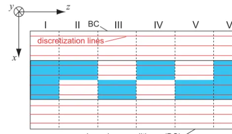
The eigenmodes in the MoL are determined after a dis-cretization with finite differences. In this section, we describe the basic algorithm. To model waveguide structures with the MoL, we first divide it into homogeneous sections with re-spect to the direction of propagation as shown in Fig. 2. Then, solutions for the homogeneous sections and the interfaces are determined.
I II III IV V VI
boundary conditions (BC) BC
discretization lines
x
z y
Figure 2. Analysis with the MoL: dividing the structure into homo-geneous sections and discretization.
boundary conditions (BC)
BC
BC
BC
x
y
z
E ,Hx y
E ,Hy x
Figure 3. Discretization points in the cross-section.
Solution in homogeneous sections
For the numerical analysis, we start with generalized trans-mission line (GTL) equations, which relate the transverse electric and magnetic fields. In what follows, the coor-dinates are normalized with the free space wave num-ber k0=ω
√
ε0µ0=2π/λ0: u=k0u (u=x, y, z). Further,
the magnetic field is normalized with the free space wave impedanceZ0=
√
µ0/ε0=120π :Heu=Z0Hu. Then, the
GTL-equations read (see e.g.Pregla, 1999; Pregla, 2008):
∂[H]t
∂z = −j RE[E]t
∂[E]t
∂z = −j RH[H]t (1)
with [E]t=
Ey
Ex
[H]t=
−
e Hx
e Hy
(2) Note: the continuous physical vectors were put in brack-ets here, to distinguish them from mathematical vectors that originate from discretization. These mathematical vectors are written in bold.
In the analysis, anisotropic materials of the following form are considered:
ν ↔
r=
νx 0 0
0 νy 0
0 0 νz
with ν
↔
r=ε
↔
r, µ
↔
S. F. Helfert: Left eigenvectors 21 With these tensors for the material parameters the
opera-torsRHundREare given as:
RE=
εy+Dxµ−z1Dx −Dxµ−z1Dy
−Dyµ−z1Dx εx+Dyµ−z1Dy
RH=
µx+Dyε−z1Dy Dyεz−1Dx
Dxε−z1Dy µy+Dxεz−1Dx
Note: in the following the derivatives in x, y direction will be treated differently than the derivative with respect to z. To indicate this, the abbreviationDv=∂/∂v(withv=x, y)
was introduced for these derivatives.
By combining the GTL-equations (1), the following cou-pled wave equations are obtained:
∂2[H]t
∂z2
−QH[H]t= [0]
∂2[E]t
∂z2
−QE[E]t= [0] (4)
with
QH= −RERH QE= −RHRE (5)
The next step of the analysis is the discretization of Eq. (4) with finite differences in the direction of the cross–section, while thez-dependency remains. Figures 2–3 show this dis-cretization process from the top and in the cross-section.
As indicated, the components of the electric or magnetic fields (i.e.Ex,Eyresp.Hx,Hy) are determined at different
positions. With this shift, the coupling between the compo-nents that is described by the product of first derivatives in
x andy direction (see off-diagonal elements ofRE,H) can
be modeled in an optimal way. [More details can be found e.g. in Pregla, 2008].
Now, the fields are combined in vectors, and the operators
Q,Rbecomes operator matrices that contain the approxima-tions of the derivatives with finite differences and the mate-rial parameters.
[H]t⇒H [E]t⇒E QH,E⇒QH,E RH,E⇒RH,E
In what follows, we describe the solution of the wave equa-tion for the electric and magnetic field in parallel. However, these fields are coupled by Eq. (1). Therefore, in practice, we have to solve the wave equation for only one of the fields and determine the remaining one with the help of Eq. (1).
After discretization, Eq. (4) becomes:
∂2H
∂z2
−QHH =0
∂2E
∂z2
−QEE=0 (6)
The expressions in Eq. (6) are coupled linear differential equation systems. As known from mathematics, such equa-tion systems can be solved by transformaequa-tion to principal axes
QE,H=TE,H02T−E,1H (7)
with TE,Hand02being the eigenvectors and eigenvalues of
QE,H.
Here, the matrices QE and QH were determined from
Eq. (5) and then discretized with finite differences. How-ever, identical matrices are obtained if the operatorsREand
RH are discretized first and the multiplication is done for
these discrete matrices. Now, as known from mathematics (see e.g. Zurmühl and Falk, 1984, pp. 163) the eigenvalues of matrices that are determined from the product of two square matrices in reversed order are identical. For this reason QE
and QHhave the same eigenvalues and the subscript E or H
was omitted for02.
After transforming the fields according to:
H=THH E=TEE (8)
a system of decoupled equations is developed:
∂2H
∂z2
−02H =0 ∂
2E
∂z2
−02E=0 (9) whose solution can be given immediately as:
E=e−0zEf+e0zEb (10)
H=e−0zHf+e0zHb (11)
Equations (7)–(11) show that the solution of the wave equa-tion is given in terms of eigenmodes. Each column of the eigenvector matrices TE,H represents the electric resp.
mag-netic fields of these eigenmodes, 0 is a diagonal matrix with the propagation constants and the overlined quantities
Ef,bHf,brepresent the amplitudes of the forward and
back-ward propagating modes. By introducing the solution for the electric or magnetic field Eqs. (10), (11) into the GTL-expressions in discretized domain Eq. (1) one can obtain fol-lowing relation between the amplitudes:
Ef=Hf Eb= −Hb (12)
In this case, the transformation matrices are related according to:
TE=jRHTH0−1 TH=jRETE0−1 (13)
Interfaces
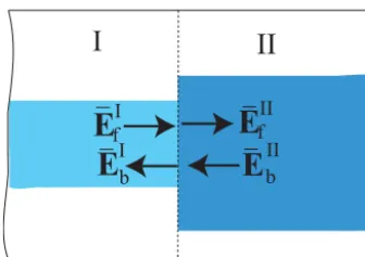
After solving the wave equation in homogeneous sections, interfaces must be considered. Here, the transverse electric and magnetic field components have to be continuous. Fig-ure 4 shows an interface between two sections (I and II) with individual eigenmodes. From the continuity condition for the
22 S. F. Helfert: Left eigenvectors
E
fIE
fIIE
IbE
bIII
II
Figure 4. Interface between two homogeneous sections.
transverse fields, a relation for the amplitudes of the eigen-modes is obtained, where Eqs. (8)–(12) were considered
TIE TIE TIH −TIH
EIf
EIb
! =
TIIE TIIE TIIH −TIIH
EIIf
EIIb
!
(14)
From Eq. (14) we can e.g. compute the amplitudes of the eigenmodes in region II from the ones in region I in the fol-lowing way:
EIIf +EIIb=aII,I(E
I f+E
I
b) (15)
EIIf −EIIb=bII,I(E
I f−E
I
b) (16)
with aII,I=(TIIE)
−1TI
E and bII,I=(TIIH)
−1TI
H (17)
In principle, we are now in position to analyze whole devices like the polarization converter shown in Fig. 1. For this pur-pose, we must introduce conditions at the input and output of the device and apply the expressions derived for the homoge-neous sections and the interfaces. However, the exponential increasing terms in Eqs. (10)–(11) can cause numerical prob-lems if e.g. transfer matrices are used. Therefore, numerical stable expressions have been developed in the past, to avoid the numerical computation of these exponential increasing terms. These are algorithms with impedances/admittances (see e.g. Rogge and Pregla, 1993; Pregla, 2008) or with scat-tering parameters (e.g. Helfert and Pregla, 2002). At this point, we do not go into details, but just refer to the relevant literature.
2.2 Reduction of the eigenmode system
The presented algorithm works well, if the number of dis-cretization lines is not too high. However, particularly if vec-torial, 3-D problems are considered, the occurring matrices for the electric/magnetic field distribution become very large. The determination of all eigenmodes in Eq. (7) is very time consuming and the memory requirement becomes very high.
For this reason, the analysis with a reduced number of eigen-modes was proposed in Gerdes (1994). However, in that pa-per all eigenmodes were determined first. Only after that, some of them were omitted for the further simulations.
In Schneider (1999) was described how this computa-tion of all eigenmodes can be avoided. For this purpose the Arnoldi algorithm that is implemented in the MATLAB pro-gram package (MATLAB, 2014) was used. This was done here as well. Information about this method can be found in the literature (e.g. Arnoldi, 1951; Golub and van Loan, 1989) so that we do not go into details here.
With a reduced set of eigenmodes the continuity of the transverse fields at interfaces leads to expressions where the matrices have the following shape:
4 S. Helfert: Left Eigenvectors
From Eq. (14) we can e.g. compute the amplitudes of the eigenmodes in region II from the ones in region I in the fol-lowing way: 135 (15) (16) with and (17)
In principle, we are now in position to analyze whole devices like the polarization converter shown in Fig. 1. For this pur-pose, we must introduce conditions at the input and output of 140
the device and apply the expressions derived for the homoge-neous sections and the interfaces. However, the exponential increasing terms in Eqs. (10)-(11) can cause numerical prob-lems if e.g. transfer matrices are used. Therefore, numerical stable expressions have been developed in the past, to avoid 145
the numerical computation of these exponential increasing terms. These are algorithms with impedances/admittances (see e.g. (Rogge and Pregla, 1993), (Pregla, 2008)) or with scattering parameters (e.g. (Helfert and Pregla, 2002)). At this point, we do not go into details, but just refer to the rele-150
vant literature.
2.2 Reduction of the eigenmode system
The presented algorithm works well, if the number of dis-cretization lines is not too high. However, particularly if vectorial, 3D problems are considered, the occurring matri-155
ces for the electric/magnetic field distribution become very large. The determination of all eigenmodes in Eq. (7) is very time consuming and the memory requirement becomes very high. For this reason, the analysis with a reduced number of eigenmodes was proposed in (Gerdes, 1994). However, in 160
that paper all eigenmodes were determined first. Only after that, some of them were omitted for the further simulations.
In (Schneider, 1999) was described how this computa-tion of all eigenmodes can be avoided. For this purpose the Arnoldi algorithm that is implemented in the MATLAB pro-165
gram package (MATLAB, 2014) was used. This was done here as well. Information about this method can be found in the literature e.g. (Arnoldi, 1951), (Golub and van Loan, 1989) so that we do not go into details here.
With a reduced set of eigenmodes the continuity of the 170
transverse fields at interfaces leads to expressions where the matrices have the following shape:
TEI
=
TEI TEII TEII
-THI
THI THII -THII
EfI
EbI
EfII
EbII
Hence, the expressions in Eq. (15)–(17) require the inver-sion of non-square matrices. The use of a pseudo-inverse (see (Strang, 1986)) was proposed in (Schneider, 1999) for 175
this purpose. Here, we follow a different path and apply left eigenvectors as described in (Helfert et al., 2003).
In principle the left eigenvectorsof a matrixare so-lutions of
(18)
in contrast to the more known problem for the right eigen-vectors
(19)
The eigenvalues for both problems are identical. After suit-able sorting and normalization of the left and right eigenvec-tors we may write:
(20)
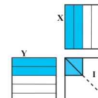
where is the identity matrix. For our purpose, it is im-portant that this relation is also true when a reduced set of eigenmodes is used. This is indicated in Fig. 5.
180
Y
X
I
Fig. 5. Multiplication of left- and right-eigenvectors resulting in an identity matrix
Note: Equation (20) is true, as long as the eigenvalues are different. For degenerated modes with identical eigenval-ues this condition does not have to be fulfilled. However as shown e.g. in Zurm¨uhl and Falk (1984), pp. 155 it is possible to transform the eigenvectors in such a way that condition 185
Eq. (20) is enforced. A summary of this transformation is given in the appendix.
Once the left eigenvectors (indicated by the superscript ’L’) have been computed, we determine the expressions given in Eq. (17) as:
and (21)
The superscript ’r’ indicates that a reduced set of eigenmodes was used. It is now worth noting that the matrices in Eq. (21) are sub-matrices of the ones given in Eq. (17). The illustra-190
tion shown in Fig. 5 can be interpreted as a special case of this feature.
Unfortunately, the author is not aware of a standard al-gorithm that determines right- and left-eigenvectors at the same time. As consequence, in the past, the right and left 195
eigenvectors were determined independently of each other Hence, the expressions in Eqs. (15)–(17) require the
inver-sion of non-square matrices. The use of a pseudo-inverse (see Strang, 1986) was proposed in Schneider (1999) for this pur-pose. Here, we follow a different path and apply left eigen-vectors as described in Helfert et al. (2003).
In principle the left eigenvectors Y of a matrix A are solu-tions of
YA=λY (18)
in contrast to the more known problem for the right eigen-vectors X
AX=Xλ (19)
The eigenvaluesλfor both problems are identical. After suit-able sorting and normalization of the left and right eigenvec-tors we may write:
YX=I (20)
where I is the identity matrix. For our purpose, it is impor-tant that this relation is also true when a reduced set of eigen-modes is used. This is indicated in Fig. 5.
Note: Eq. (20) is true as long as the eigenvalues are differ-ent. For degenerated modes with identical eigenvalues this condition does not have to be fulfilled. However as shown e.g. in Zurmühl and Falk (1984), pp. 155 it is possible to transform the eigenvectors in such a way that condition Eq. (20) is enforced. A summary of this transformation is given in the Appendix.
Once the left eigenvectors (indicated by the superscript “L”) have been computed, we determine the expressions given in Eq. (17) as:
S. F. Helfert: Left eigenvectors 23 The superscript “r” indicates that a reduced set of
eigen-modes was used. It is now worth noting that the matrices in Eq. (21) are sub-matrices of the ones given in Eq. (17). The illustration shown in Fig. 5 can be interpreted as a special case of this feature.
Unfortunately, the author is not aware of a standard al-gorithm that determines right- and left-eigenvectors at the same time. As consequence, in the past, the right and left eigenvectors were determined independently of each other (Helfert et al., 2003). This was done with QE,Hand its
trans-posed. Obviously, the numerical effort is quite high. As sec-ond problem the numerical orthogonality of the left and right eigenvectors Eq. (20) can be quite bad when they are com-puted independently.
2.3 Efficient determination of the left eigenvectors In this section we describe how we can avoid solving the eigenvalue problem twice. To develop suitable expressions, we start with the operatorsRE,H. For Dirichlet, Neumann, or
periodic boundary conditions, we may write the discretized operators with matrix products of the following form:
RE=
"
εy−DTxµ−1
z Dx −DTxµ
−1 z DTy
−Dyµ−z1Dx εx−Dyµ−z1DTy
#
(22)
RH=
"
µx−Dyε−z1DTy −Dyε
−1 z DTx
−Dxε−z1DTy µy−Dxε−z1DTx
#
(23)
The matrices Dx, Dy and their transposed (indicated by the
superscript “T”) contain the finite difference approximation of the derivatives with respect tox andy.εx,y,z andµx,y,z
are diagonal matrices containing the permittivities and per-meabilities on the discretization points. As can be seen, the matrices are symmetric (not Hermitian)
RTE,H=RE,H (24)
Next we look at the matrices that occur in the wave equation Eq. (6). As mentioned before, we may write
QH= −RERH QE= −RHRE
If we now transpose e.g. QH, we find, due to Eq. (24), the
following relation:
QTH= −(RERH)T= −RTHRTE= −RHRE=QE (25)
Next, this transposed matrix is diagonalized. We use the left eigenvector matrix (indicated by the superscript “L”, as be-fore) as inverse of THand obtain
QTH=(TH02TLH) T=(TL
H) T02TT
H (26)
Similar, the diagonalization of QEreads:
QE=TE02TLE (27)
Y
X
I
Figure 5. Multiplication of left- and right-eigenvectors resulting in an identity matrix.
A comparison of Eq. (26) and Eq. (27) with consideration of Eq. (25) shows that TE, TH and the corresponding left
eigenvectors (i.e. their inverse matrices) are related according to:
TTE=TLH TTH=TLE (28)
Note: since eigenvectors can be determined up to an arbitrary scaling factor, Eq. (28) is only true, if the eigenvectors have been normalized accordingly. This is not a principle problem, but has to be kept in mind.
As final step we introduce Eq. (28) into Eq. (13) and ob-tain:
(TLH)T=jRHTH0−1 (TLE)T=jRETE0−1 (29)
The products in Eq. (29) can be computed with verly low numerical effort, because RH and RE are sparse–matrices.
Further, the eigenvalues are combined in the diagonal matrix
0 so that its inverse can be computed very easily. Hence, Eq. (29) shows that the left eigenvectors can be determined with simple matrix products from the previously determined right eigenvectors. The numerical effort for this procedure is clearly lower than that for solving the eigenvalue/eigenvector problem twice or as determining a pseudo inverse.
2.4 Open structures
As mentioned before, the derived expression Eq. (29) only holds for special boundary conditions, for which the operator matrices RE,Hare symmetric. Now outgoing waves are
com-pletely reflected at Dirichlet or Neumann boundaries (“hard boundaries”) leading to modeling errors. There exist vari-ous ways to reduce such reflections, e.g. absorbing boundary conditions (ABC) as described in Pregla (1995) or Vassallo and Collino (1997). Unfortunately, with the ABCs mentioned above, the symmetry condition in Eq. (24) does not hold any longer. Hence, we need to apply methods that permit the in-clusion of hard BCs.
Particularly, we decided to use perfectly matched layers (PMLs). These are lossy layers positioned at the boundary of the computational window. Waves that enter this region are damped and after being reflected at the hard wall, they are
24 S. F. Helfert: Left eigenvectors damped further to negligible amplitudes before re-entering
the original computational window.
Generally, PMLs can be interpreted in various ways (see e.g. Berenger, 1994; Mittra and Pekel, 1995; Rappaport, 1995; Al-Bader and Jamid, 1998). Here, they are considered as lossy anisotropic layers, which are described by tensors that only contain non-zero elements on the main diagonal (see e.g. Sacks et al., 1995; Werner and Mittra, 1997; Cu-cinotta et al., 1999), i.e. tensors of the form given by Eq. (3), for which the formulas were derived. Hence, Eq. (29) is also true for PMLs.
2.4.1 Orthogonality of the eigenmodes
By considering the conservation of energy and from the reci-procity theorem one can derive orthogonality relations for the eigenmodes in waveguide sections (see e.g. Syms and Coz-ens, 1992; Snyder and Love, 1983). For the fields of two dif-ferent eigenmodes (labelsi, k) that propagate inzdirection the orthogonality condition reads
Z Z
A
([E]i× [H]k)· [e]zdA=0 (30)
Note: as before, the physical vectors ([E],[H],[e]) were writ-ten in brackets.
In the MoL, the discretized field distributions of the eigen-modes are combined in the columns of the matrices TE, TH.
Therefore, the discretized integral in Eq. (30) contains the product
(TH)T·(TE)
which results in a diagonal matrix, as derived. Hence, the or-thogonality of the discretized eigenmodes in a closed struc-ture can be seen directly from Eq. (28). We should point out that this orthogonality relation does also hold for lossy struc-tures.
3 Numerical results
In this section we show some numerical examples to evaluate the derived expression. For comparison the left eigenvectors were (a) determined with Eq. (29) and (b) by solving a sec-ond eigenvalue/eigenvector problem as described in (Helfert et al., 2003). For a quantitative assessment, an error measure was introduced. Ideally, the product between left- and right-eigenvectors results in an identity matrix. The deviation from this ideal result can be written as:
TLTR=I+Merr (31)
In the following we will use ||Merr||max i.e. the maximum element of this matrix as error measure.
There are a few factors that contribute to this error. The first one is caused by the finite machine precision so that the
eigenvectors can be determined only up to a certain accuracy. A second contribution to the error comes from degenerated eigenmodes, as mentioned in Sect. 2.2. As will be shown nu-merically in this section this error can be reduced by a trans-formation of these modes.
To see if the developed expressions work in principle and to study the behavior of the PMLs, we started with two sim-ple 2-D structures (TE-polarization with the componentsEy,
Hx,Hz). For both cases Dirichlet conditions were introduced
at the lateral boundaries and results obtained with and with-out PMLs were compared. As mentioned before, the PMLs were introduced as anisotropic materials (18 lines close to the boundaries) where the following values for the materi-als were chosen:µz=εy=1−0.36j,µx=1/µz. For
de-tails about the relation between these values see e.g. Sacks et al. (1995), Werner and Mittra (1997), and Cucinotta et al. (1999).
We should point out that thezdirection is treated with ana-lytic expressions. Hence, to model the infinite long structures no PMLs are needed, but we assume that only forward propa-gating modes occur for these regions in Eqs. (10)–(11), thus:
Eb=Hb=0. Since we are dealing with 2-D problems, a
reduction of the eigenmode system is not necessary, and all eigenmodes were used for the computations. Particularly, the number of discretization points (=number of eigenmodes) was 107.
First of all, a tilted Gaussian beam was injected into a ho-mogeneous air region. The input field is given as:
Eyin(x, z=0)=E0e−(x/w)
2
e−j k0xcos(ϕ) (32)
withλ0=1.55 µm,w=2 µm andϕ=45◦. To compute the
wave propagation of the Gaussian beam, we discretize the input field inxdirection and must invert Eq. (8) after that. As mentioned before, an infinite long region with only forward propagating modes is assumed. Hence, the inversion (written with left eigenvectors) reads:
Ef in=TLEEin (33)
In the following, the propagation in the region is com-puted with Eq. (10) and the original fields are obtained from Eq. (8). As can be seen, even in this simple case left eigen-vectors are used.
As second example the abrupt ending of a waveguide was studied. As can be seen in Fig. 6, we have the concatena-tion of a waveguide secconcatena-tion and an infinite long air region. In the simulations the fundamental waveguide mode was in-jected on the left. Then, the wave propagation was simulated with the expressions given in Sect. 2. For this structure the left eigenvectors were needed to enforce the continuity of the fields at the interface between the waveguide and the air region.
S. F. Helfert: Left eigenvectors 25
PML
PML
n =1
n =1.4
Figure 6. Abrupt ending of a waveguide.
Table 1. Error determined with Eq. (31) for the structures shown in Fig. 6; in case “PML symmetric a)” the eigenmodes were taken as obtained by the eigenvalue procedure; in “PML symmetric b)” the degenerated eigenmodes were transformed.
ncore 1.4 1.4−0.01j
electric wall 10−12 10−11 PML
symmetric a) 0.15 0.7 symmetric b) 10−9 10−9 PML
asymmetric 10−11 10−11
the worse one was taken. Since the homogeneous air region is already included in these studies, there are no additional error measures required for the Gaussian beam problem.
In the simulations, several parameters were varied. We should repeat that the expression in Eq. (29) was derived for a general case incl. losses. These losses can be caused by dielectric media (i.e. with complex permittivity) or by PMLs (anisotropic media with complex permittivity and permeabil-ity). Hence, the influence of the losses on the error is of par-ticular interest.
The results for the error are summarized in Table 1. As can be seen, two cases were compared; for a lossless core (ncore=1.4) and a lossy one (ncore=1.4–0.01j). The
lossless case (row “electric wall”) leads to the small error ||Merr||max=10−12, which deteriorates only moderately for a lossy core.
The next rows show the influence of the PMLs on the er-ror. In row “PML symmetric a)” the determined error-value was computed directly after determining the right and left eigenvectors with Eqs. (7) and (29). Here, degenerated eigen-modes (i.e. pairs with identical propagation constant) occur, resulting in very high error values. This error can be reduced drastically by a transformation of the eigenmodes leading to the results ”symmetric b)”.
Since the error in case of PMLs is caused by degener-ated modes, it was examined next, what happens if a small
S. Helfert: Left Eigenvectors
7
lossless case (row ” electric wall”) leads to the small error
, which deteriorates only moderately
for a lossy core.
a)
0 1 2 3 4 5 6 7 8 9 10 0.2 0.4 0.6 0.8 1.0 1.2 1.4 −5 −4 −3 −2 −1 0 1 2 3 4 5 x [μm]
z [μm]
b) 0.1 0.2 0.3 0.4 0.5 0.6 0.7 0.8 0.9 1.0 −5 −4 −3 −2 −1 0 1 2 3 4 5 x [μm]
0 1 2 3 4 5 6 7 8 9 10
z [μm]
Fig. 7. Injection of a tilted Gaussian beam into a homogeneous section, computed electric field, a) without PMLs, b) with PMLs, the horizontal lines indicate the boundaries of the PMLs
1.4 electric wall PML
symmetric a) 0.15 0.7
symmetric b) PML asymmetric
Table 1. Error determined with Eq. 31 for the structure shown in Fig. 6; in case ’PML symmetric a)’ the eigenmodes were taken as obtained by the eigenvalue procedure; in ’PML symmetric b)’ the degenerated eigenmodes were transformed
The next rows show the influence of the PMLs on the error.
315
In row ”PML symmetric a)” the determined error-value was
computed directly after determining the right and left
vectors with Eqs. (7) and (29). Here, degenerated
eigen-modes (i.e. pairs with identical propagation constant) occur,
resulting in very high error values. This error can be reduced
320
drastically by a transformation of the eigenmodes leading to
the results ”symmetric b)”.
a) 0.1 0.2 0.3 0.4 0.5 0.6 0.7 0.8 0.9 1.0 −5 −4 −3 −2 −1 0 1 2 3 4 5 x [μm]
0 2 4 6 8 10 12 14 16 18 20
z [μm]
b)
0 2 4 6 8 10 12 14 16 18 20 0.1 0.2 0.3 0.4 0.5 0.6 0.7 0.8 0.9 1.0 1.1 −5 −4 −3 −2 −1 0 1 2 3 4 5 x [μm]
z [μm]
Fig. 8. Electric field in the structure shown in Fig. 6; a) without PMLs, b) PMLs included, the horizontal lines indicate the bound-aries of the PMLs
Since the error in case of PMLs is caused by degenerated
modes, it was examined next, what happens if a small
asym-metry in the PMLs is introduced. In particular, on the lower
325
boundary, the imaginary part of
was increased by the
fac-tor 1.0001 and the other values (
,
) were modified
ac-cordingly. Then, the degeneration of the modes vanishes,
leading to the error presented in row: ”PML asymmetric”.
These errors are close to the lossless case.
330
Keeping in mind that the values in row ”PML symmetric
a)” can be improved to ”PML symmetric b)”, it is found that
all errors are quite small. Hence the formulas Eq. (31) work
without problems for the 2D-case incl. losses due to lossy
materials or PMLs.
335
For comparison, the left eigenvectors were also
deter-mined from solving a second eigenvalue problem. Here, the
error for the lossless case is reduced to
. For all other
cases, however, the error is similar or slightly higher than
given in Table-1.
340
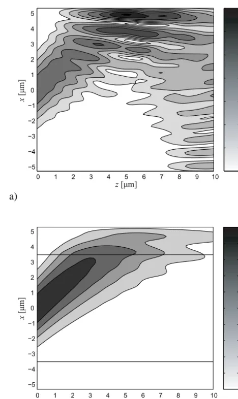
Figure 7. Injection of a tilted Gaussian beam into a homogeneous section, computed electric field, (a) without PMLs, (b) with PMLs, the horizontal lines indicate the boundaries of the PMLs.
asymmetry in the PMLs is introduced. In particular, on the lower boundary, the imaginary part ofµz was increased by
the factor 1.0001 and the other values (εy,µx) were modified
accordingly. Then, the degeneration of the modes vanishes, leading to the error presented in row: “PML asymmetric”. These errors are close to the lossless case.
Keeping in mind that the values in row “PML symmetric a)” can be improved to “PML symmetric b)”, it is found that all errors are quite small. Hence the formulas Eq. (31) work without problems for the 2-D-case incl. losses due to lossy materials or PMLs.
For comparison, the left eigenvectors were also deter-mined from solving a second eigenvalue problem. Here, the error for the lossless case is reduced to 10−15. For all other cases, however, the error is similar or slightly higher than given in Table 1.
26 S. F. Helfert: Left eigenvectors
S. Helfert: Left Eigenvectors
7
lossless case (row ” electric wall”) leads to the small error
, which deteriorates only moderately
for a lossy core.
a)
0 1 2 3 4 5 6 7 8 9 10 0.2 0.4 0.6 0.8 1.0 1.2 1.4 −5 −4 −3 −2 −1 0 1 2 3 4 5 x [μm] z [μm] b) 0.1 0.2 0.3 0.4 0.5 0.6 0.7 0.8 0.9 1.0 −5 −4 −3 −2 −1 0 1 2 3 4 5 x [μm]
0 1 2 3 4 5 6 7 8 9 10
z [μm]
Fig. 7. Injection of a tilted Gaussian beam into a homogeneous section, computed electric field, a) without PMLs, b) with PMLs, the horizontal lines indicate the boundaries of the PMLs
1.4 electric wall PML
symmetric a) 0.15 0.7
symmetric b) PML asymmetric
Table 1. Error determined with Eq. 31 for the structure shown in Fig. 6; in case ’PML symmetric a)’ the eigenmodes were taken as obtained by the eigenvalue procedure; in ’PML symmetric b)’ the degenerated eigenmodes were transformed
The next rows show the influence of the PMLs on the error.
315
In row ”PML symmetric a)” the determined error-value was
computed directly after determining the right and left
eigen-modes (i.e. pairs with identical propagation constant) occur,
resulting in very high error values. This error can be reduced
320
drastically by a transformation of the eigenmodes leading to
the results ”symmetric b)”.
a) 0.1 0.2 0.3 0.4 0.5 0.6 0.7 0.8 0.9 1.0 −5 −4 −3 −2 −1 0 1 2 3 4 5 x [μm]
0 2 4 6 8 10 12 14 16 18 20
z [μm]
b)
0 2 4 6 8 10 12 14 16 18 20 0.1 0.2 0.3 0.4 0.5 0.6 0.7 0.8 0.9 1.0 1.1 −5 −4 −3 −2 −1 0 1 2 3 4 5 x [μm]
z [μm]
Fig. 8. Electric field in the structure shown in Fig. 6; a) without PMLs, b) PMLs included, the horizontal lines indicate the bound-aries of the PMLs
Since the error in case of PMLs is caused by degenerated
modes, it was examined next, what happens if a small
asym-metry in the PMLs is introduced. In particular, on the lower
325
boundary, the imaginary part of
was increased by the
fac-tor 1.0001 and the other values (
,
) were modified
ac-cordingly. Then, the degeneration of the modes vanishes,
leading to the error presented in row: ”PML asymmetric”.
These errors are close to the lossless case.
330
Keeping in mind that the values in row ”PML symmetric
a)” can be improved to ”PML symmetric b)”, it is found that
all errors are quite small. Hence the formulas Eq. (31) work
without problems for the 2D-case incl. losses due to lossy
materials or PMLs.
335
For comparison, the left eigenvectors were also
deter-mined from solving a second eigenvalue problem. Here, the
error for the lossless case is reduced to
. For all other
cases, however, the error is similar or slightly higher than
Figure 8. Electric field in the structure shown in Fig. 6; (a) withoutPMLs, (b) PMLs included, the horizontal lines indicate the bound-aries of the PMLs.
The computed electric field distributions are presented in Fig. 7 for the Gaussian beam and in Fig. 8 for the abrupt end-ing of the waveguide. The PML-graphs were obtained with symmetric PMLs. However, there are no visual differences recognizable when a small asymmetry is introduced.
For both structures it can be seen, how the reflections caused by the Dirichlet boundaries Fig. 7a (resp. Fig. 8a) can be suppressed with the PMLs Fig. 7b (resp. Fig. 8b).
The results presented so far show that the algorithm works in principle in 2-D including losses. However, the analysis of such a 2-D-structures is numerical not very demanding and (as was done) the full eigenmode system can be used.
Therefore, the real reduction of the numerical effort is ex-pected for 3-D-structures. Two examples were considered here.
w
d
y xd
xw
ymetal
air
Figure 9. Array of hollow waveguides; dimensions:wx=0.8λ0 wy=0.6λ0,dx=dy=0.04λ0, with the free space wavelengthλ0.
The polarization converter shown in Fig. 2 had already been examined with the MoL (Helfert et al., 2003). In that study the left eigenvectors were determined from an inde-pendent eigenvalue/eigenvector computation. The structure was analyzed withNx×Ny×2=100×75×2=15 000
dis-cretization points (factor “2” because of the vectorial anal-ysis) and 300 eigenmodes. When the left eigenvectors were determined with the algorithm described here, the value 10−8 was obtained for the error Eq. (31). The separate left eigen-vector determination (Helfert et al., 2003) results in the error value 10−7. Both values are satisfactory. We should point out here, that most of the CPU-time for analyzing the polariza-tion converter is required for the determinapolariza-tion of the eigen-modes. In particular, computing the left eigenvectors sepa-rately, required 3 min, which could be reduced to 4 s with the algorithm presented here (computations on a PC). This shows the significant reduction of the numerical effort.
The features of this polarization converter had been stud-ied with the MoL in detail in (Helfert et al., 2003). Since these results do not change, when the eigenvectors are de-termined differently, they are not repeated here. Instead we refer to Helfert et al. (2003).
As second example for a 3-D-device, an array of hollow waveguides as shown in Fig. 9 was examined. The idea is to use such hollow waveguide arrays as polarization converting elements. For this purpose, the difference of the propagation constants of the vertically and horizontally polarized eigen-modes is utilized (“half–wave plate”) and the lengthLzof the
device was chosen in such a way that these wave experience a phase difference ofπ. Hence:
k01neffLz=π (34)
A detailed description of the structure is given in Helfert et al. (2014) and Helfert et al. (2015). Therefore, we concentrate here on the results as far as the numerical algorithm is con-cerned and do not repeat all the features of this device.
S. F. Helfert: Left eigenvectors 27
Figure 10. Injection of a plane wave into an array of hollow waveg-uides, magnetic field in front of the waveguides.
metal. Its relative permittivity was determined with a Dude-model, resulting in:
– THz (λ0=0.48 mm,f=0.625 THz)
εrAg= −6.2×10⁵−2.25×10⁶j
– Optics (λ0=1000 nm,f =3×10¹⁴Hz)
εrAg= −47−1.89j
As can be seen, losses in the metal are considered.
With the values for the permittivity given above, the eigen-modes were computed. Then, the following lengths were de-termined from Eq. (34):
LzTHz=2.2λ0 Lzoptics=3λ0 (35)
Now, plane waves were injected into the structures as shown in Fig. 10. The magnetic field at the output is sketched in Fig. 11. The rotation of the fields is clearly seen. In the THz case (Fig. 11a) we recognize that the whole field is in-side the air-region, whereas a non–negligible part of the field is inside the metal in optics (Fig. 11b).
The computations were done withNx×Ny×2=170×
130×2=44 200 discretization points. The number of eigen-modes was 20 i.e. much lower. With these parameters, the following error values occur:||Merr||max=10−9(THz), ||Merr||
max=10−8(optics). When the left eigenvectors were
determined separately (see (Helfert et al., 2003)), errors of the same order were obtained. So, Eq. (29) does also work very well for the considered full vectorial 3-D-structures.
4 Summary and conclusions
In this paper was shown how left eigenvectors can be deter-mined very efficiently. For this purpose the relation between the transverse electric and magnetic fields of the eigenmodes was utilized. It was found that the matrix of the left eigenvec-tors can be computed by simple matrix products from pre-viously determined right eigenvalues in case of hard walls
S. Helfert: Left Eigenvectors 9
a)
b)
Fig. 11. Magnetic field at the output of the hollow waveguides, a) THz-frequencies, b) optics
The computations were done with!
!
discretization points. The number of eigen-395
modes was 20 i.e. much lower. With these parameters, the following error values occur:
$ (THz),
(optics). When the left eigenvectors were determined separately (see (Helfert et al., 2003)), errors of the same order were obtained. So, Eq. (29) does also work 400
very well for the considered full vectorial 3D-structures.
4 Summary and conclusions
In this paper was shown how left eigenvectors can be deter-mined very efficiently. For this purpose the relation between the transverse electric and magnetic fields of the eigenmodes 405
was utilized. It was found that the matrix of the left eigenvec-tors can be computed by simple matrix products from pre-viously determined right eigenvalues in case of hard walls (Dirichlet, Neumann) or periodic boundaries. Compared to the erlier determination from a second eigenvalue problem, 410
the numerical effort could be reduduced significantly. Absorbing boundary condition that are often employed in the MoL, cannot be used here, because of symmetry
require-ments. Therefore, open structures were modeled with per-fectly matched layers where the PMLs were introduced as 415
lossy anisotropic materials. The numerical results (incl. er-ror measures) for various structures in 2D and for 3D show that the method works very well also when losses are consid-ered.
Appendix A 420
If multiple eigenmodes with identical propagation constant are computed, Eq. (20) does not necessarily hold. However, as described e.g. in (Zurm¨uhl and Falk, 1984), it is always possible to transform the corresponding eigenvectors to en-force this conditions. Here, we will briefly repeat the pro-cedure given in (Zurm¨uhl and Falk, 1984). In what follows,
and
are the submatrices of the right and left eigen-vector matrix that correspond to the multiple eigenvalues. Generally, their product results in a full matrix:
(A1)
Note: in this paper the left eigenvectors were introduced as row-vectors. This is in contrast to (Zurm¨uhl and Falk, 1984) where they were written as column vectors. So, some of the expressions in (Zurm¨uhl and Falk, 1984) are transposed com-pared to the formulas given here.
425
Now, the eigenvectors are transformed in the following way:
(A2)
where the new eigenvectors are orthogonal:
(A3)
Then one can write
(A4)
Hence, the matrices and
must be chosen such that their product gives. This choice is not unique. The use of triangular matrices was proposed in (Zurm¨uhl and Falk, 1984) and as second possibility chosing
(or
) was mentioned. Due to Eq. (29) we chose here:
(A5)
resulting in the following expression
(A6)
to compute
. We should point out that the size of (i.e. the number of eigenmodes with identical eigenvalues) is usu-ally very small. (For the structures examined in this paper the maximum size was 4). Therefore, the numerical effort for solving Eq. (A6) is negligible.
430 Figure 11. Magnetic field at the output of the hollow waveguides, (a) THz-frequencies, (b) optics.
(Dirichlet, Neumann) or periodic boundaries. Compared to the erlier determination from a second eigenvalue problem, the numerical effort could be reduduced significantly.
Absorbing boundary condition that are often employed in the MoL, cannot be used here, because of symmetry require-ments. Therefore, open structures were modeled with per-fectly matched layers where the PMLs were introduced as lossy anisotropic materials. The numerical results (incl. error measures) for various structures in 2-D and for 3-D show that the method works very well also when losses are considered.
28 S. F. Helfert: Left eigenvectors Appendix A
If multiple eigenmodes with identical propagation constant are computed, Eq. (20) does not necessarily hold. However, as described e.g. in (Zurmühl and Falk, 1984), it is always possible to transform the corresponding eigenvectors to en-force this conditions. Here, we will briefly repeat the proce-dure given in (Zurmühl and Falk, 1984). In what follows, Xm
and Ymare the submatrices of the right and left eigenvector
matrix that correspond to the multiple eigenvalues. Gener-ally, their product results in a full matrix M:
YmXm=M (A1)
Note: in this paper the left eigenvectors were introduced as row-vectors. This is in contrast to (Zurmühl and Falk, 1984) where they were written as column vectors. So, some of the expressions in (Zurmühl and Falk, 1984) are transposed com-pared to the formulas given here.
Now, the eigenvectors are transformed in the following way:
Ym=cyeYm Xm=eXmcx (A2)
where the new eigenvectors are orthogonal: e
YmeXm=I (A3)
Then one can write
M=YmXm=cyeYmeXmcx=cycx (A4)
Hence, the matrices cy and cx must be chosen such that
their product gives M. This choice is not unique. The use of triangular matrices was proposed in (Zurmühl and Falk, 1984) and as second possibility chosing cy=I (or cx=I)
was mentioned. Due to Eq. (29) we chose here:
cy=cx (A5)
resulting in the following expression
c2x=M (A6)
to compute cx. We should point out that the size of M (i.e.
S. F. Helfert: Left eigenvectors 29 References
Al-Bader, S. and Jamid, H. A.: Perfectly matched layer absorbing boundary conditions for the method of lines modeling scheme, IEEE Microwave Guided Wave Lett., 8, 357–359, 1998. Arnoldi, W.: The Principle of minimized iterations in the solution
of the matrix eigenvalue problem, Quarterly Appl. Mathem., 9, 17–29, 1951.
Berenger, J.-P.: A perfectly matched layer for the absorption of elec-tromagnetic waves, J. Computat. Phys., 114, 185–200, 1994. Cucinotta, A., Pelosi, G., Selleri, S., Vincetti, L., and Zoboli, M.:
Perfectly matched anisotropic layers for optical waveguide anal-ysis through the finite element beam propagation method, Mi-crow. Opt, Tech. Lett., 23, 67–69, 1999.
Gerdes, J.: Bidirectional eigenmode propagation analysis of optical waveguides based on method of lines, Electron. Lett., 30, 550– 551, 1994.
Golub, G. H. and van Loan, C. F.: Matrix computations, Johns Hop-kins University Press, Baltimore, USA, 501–502, 1989. Helfert, S. F. and Pregla, R.: The method of lines: a versatile tool
for the analysis of waveguide structures, Electromagnetics, 22, 615–637, invited paper for the special issue on “Optical wave propagation in guiding structures”, 2002.
Helfert, S. F., Barcz, A., and Pregla, R.: Three-dimensional vectorial analysis of waveguide structures with the method of lines, Opt. Quantum Electron., 35, 381–394, 2003.
Helfert, S. F., Edelmann, A., and Jahns, J.: Hollow waveguides as polarization converting elements, in: Europ. Opt. Soc. ann. meet. (EOSAM), p. TOM5 S02: Subwavelength device, Berlin, Ger-many, 2014.
Helfert, S. F., Edelmann, A., and Jahns, J.: Hollow waveguides as polarization converting elements: a theoretical study, J. Europ. Opt. Soc.: Rap. Publ., 10, 15006, 1–7, 2015.
MATLAB: version 8.4 (R2014b), The MathWorks Inc., Natick, Massachusetts, 2014.
Mittra, R. and Pekel, Ü.: A new look at the perfectly matched layer (PML) concept for the reflectionless absorption of electro-magnetic waves, IEEE Microwave Guided Wave Lett., 5, 84–86, 1995.
Mustieles, F. J., Ballesteros, E., and Hernández-Gil, F.: Multimodal analysis method for the design of passive TE/TM converters in integrated waveguides, IEEE Photonics Technol. Lett., 5, 809– 811, 1993.
Pregla, R.: MoL-BPM Method of lines based beam propagation method, in: Methods for modeling and simulation of guided-wave optoelectronic devices (PIER 11), edited by: Huang, W. P., Progress in Electromagnetic Research, 51–102, EMW Publish-ing, Cambridge, Massachusetts, USA, 1995.
Pregla, R.: Novel FD-BPM for optical waveguide structures with isotropic or anisotropic material, in: Europ. Conf. Int. Opt. (ECIO), 55–58, Torino, Italy, 1999.
Pregla, R.: Analysis of electromagnetic fields and waves - The method of lines, Wiley & Sons, Chichester, UK, 2008.
Pregla, R. and Pascher, W.: The method of lines, in: Numerical tech-niques for microwave and millimeter wave passive structures, edited by: Itoh, T., 381–446, J. Wiley Publ., New York, USA, 1989.
Rappaport, C. M.: Perfectly matched absorbing boundary condi-tions based on anisotropic lossy mapping of space, IEEE Mi-crowave Guided Wave Lett., 5, 90–92, 1995.
Rogge, U. and Pregla, R.: Method of lines for the analysis of dielec-tric waveguides, J. Lightwave Technol., 11, 2015–2020, 1993. Sacks, Z. S., Kingsland, D. M., Lee, R., and Lee, J.-F.: A perfectly
matched anisotropic absorber for use as an absorbing boundary, IEEE Trans. Antennas. Propagation, 43, 1460–1463, 1995. Schneider, V. M.: Analysis of passive optical structures with an
adaptive set of radiation modes, Opt. Comm., 160, 230–234, 1999.
Snyder, A. W. and Love, J. D.: Optical waveguide theory, Chapman and Hall, London, New York, 604–605, 1983.
Strang, G.: Linear algebra and its applications, Saunders HBJ Col-lege Publishers, Orlando, Fl., USA, 3rd edn., 130–138, 1986. Sudbø, A. S.: Film mode matching: A versatile method for mode
field calculations in dielectric waveguides, Pure Appl. Opt., 2, 211–233, 1993.
Syms, R. and Cozens, J.: Optical guided waves and devices, McGraw-Hill Publishing Co., New York, chap. 6.5, 1992. Sztefka, G.: A bidirectional propagation algorithm for large
refrac-tive index steps and systems of waveguides based on the mode matching method, in: OSA Integr. Photo. Resear. Tech. Dig., 134–135, New Orleans, Louisiana, USA, 1992.
Taflove, A.: The finite-difference time–domain method, Computa-tional electrodynamics, Artech house, inc, Norwood, MA, 1995. Vassallo, C. and Collino, F.: Comparison of a few transparent boundary bonditions for finite-difference optical mode-solvers, J. Lightwave Technol., 15, 397–402, 1997.
Werner, D. H. and Mittra, R.: A new field scaling interpretation of Berenger’s PML and its comparison to other PML formulations, Microw. Opt. Tech. Lett., 16, 103–106, 1997.
Zurmühl, R. and Falk, S.: Matrizen und ihre Anwendungen, Teil 1, Springer Verlag, Berlin, Germany, 5 edn., 1984.