R E S E A R C H
Open Access
Optimal test design for binary response
data: the example of the fish embryo
toxicity test
Nadia Keddig
1*, Sophia Schubert
1and Werner Wosniok
2Abstract
Background:The fish embryo toxicity test (FET) is an established method in toxicology research for quantifying the risk potential of environmental contaminations and other substances. The typical results of the method are the half maximal effective concentration (EC50) or the no observed effect concentration (NOEC). However, from an environmental perspective, it is most important to safely identify the concentration of the substance effect which lies above the effect under control condition (spontaneous effect). The common FET is not optimal to detect ECs for small target effects. This paper shows how to optimize the efficiency and consequently the benefit of the FET for small effects using an adequate experimental design. The approach presented here can be carried over to all test systems generating binary (yes/no) outcomes.
Results:The experimental design has three components in this context: determination of spontaneous response, sample size calculation, and dose allocation. A strategy for all three components is proposed from which a design is given including precision requirements and makes the most effective use of the experimental effort. This strategy amounts to expanding the usual FET guidelines of Organisation for Economic Co-operation and Development, German Institute for Standardization, or American Society for Testing and Materials by adding a planning step that adapts the test to the specific user’s need.
Conclusions:For the practical calculation of an adapted design, a newly developed software is presented as R package
toxtestD. It provides a user-friendly way of developing an optimal experimental design for the FET without in-depth statistical knowledge. The programme is suited for all experimental problems involving a binary outcome and a continuous concentration.
Keywords:Toxicity test planning; R statistic package; Zebrafish embryo; Spontaneous lethality; Sample size; Dose design
Background
Toxicity tests in ecotoxicology serve to detect and quan-tify toxic properties of chemical substances. Typically, a toxicity test is a laboratory test, which means that the experimenter chooses the test procedure, the number of subjects to test, the doses or concentrations to apply, as well as the appropriate way to quantify toxicity. Such quantifications are used to set thresholds for allowable concentrations in the environment. Choices in experi-mental design should ensure high quality of the results in terms of precise and unbiased toxicity quantification
and of statistical decisions with controlled error rates. The design should also make optimal use of the experi-mental effort. A proper experiexperi-mental design is frequently demanded, but only a few publications on risk assess-ment deal with this aspect in detail. In this paper we use the fish embryo toxicity test (FET) as an example to demonstrate how to design a toxicity experiment attain-ing the required precision of results. We also include considerations on how to quantify toxicity using the FET results. The procedure proposed involves a four-parameter logistic dose-response model, which allows incorporating spontaneous effects as well as non-effects due to an insusceptible subpopulation. For the numerical operations of planning and analysis, we provide the R * Correspondence:[email protected]
1
Institute of Fisheries Ecology, Thünen Institute (TI), Palmaille 9, 22767 Hamburg, Germany
Full list of author information is available at the end of the article
package toxtestD, whose reference manual can be down-loaded from the CRAN homepage [1, 2].
In recent years, FET has predominantly replaced the fish acute toxicity test [3, 4]. Research projects like DanTox favour the embryos of the model organism Danio rerioto identify toxicity processes [5]. The classical version of the FET is established in research laboratories as well as in ser-vice laboratories [6–8].
A core component of the FET is exposing fertilized eggs, preferentially from zebrafish (D. rerio), in an early stage of cell division to an aquatic compound, which is charged with harmful substances. Responses to the tested substance can be death, coagulation, lethal or sublethal malformations, or teratogenic effects. The presence of effects is examined after 48 or 96 h post fertilization (hpf) [9, 4]. This test setup is used because early life stages are more sensitive than the adult life stage. In addition, early life stage tests operate fas-ter than tests on full-grown parental fishes [10]. Following the norm of the German Institute of Standardization (DIN), ten fertilized, normally developed eggs per concen-tration and a negative control should be tested [4]. The Organisation for Economic Co-operation and Development (OECD) guideline recommends 20 eggs per test concentra-tion and positive control, respectively, and 24 eggs per
negative control [9]. Both guidelines accept up to 10 % spontaneous deaths among negative controls [4, 9].
Effect quantification
Effect quantification means expressing the toxicity of a substance by a single number. The full information about the relation between concentration and toxicity (effect) is described by the concentration-response rela-tion (see example in Fig. 1a). A major concept of effect quantification is the no observed effect concentration (NOEC). It is the result of comparing observed effects in treated groups to the effects observed in the control group. The other major effect quantification is the effective concentration value (ECxx). It denotes the concentration
which causes an effect of xx %. Depending on its applica-tion, ECxx has been varyingly labelled as effective dose
(EDxx), lethal concentration/dose (LCxx/LDxx), benchmark
dose (BMD), or virtual safe dose (VSD, for very small xx) (OECD 2013 [11]). Both concepts differ clearly with regard to their properties and interpretation.
NOEC, the controversial legacy
As stated by the guidance for the implementation of REACH (Registration, Evaluation, Authorisation and
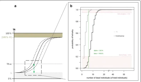
Fig. 1Sample size calculation. Logistic distribution of a concentration-response relationship (line) with a confidence interval (dotted linesaround).
Restriction of Chemicals), the NOEC is ‘the highest tested concentration for which there is no statistical sig-nificant difference of effect when compared to the con-trol group’ [12]. Similar to other statistical tests, the test sequence leading to the NOEC will detect a substance-related effect with a given safety only if it has a certain size. The detectable size and the probabil-ity of detection depend on sample size, the number of concentration points, and their allocation. Changing the sample size may shift the NOEC value over the whole range of tested concentrations, e.g. if a test se-quence is repeated with the identical set of concentra-tions, but with a different number of replicates per concentration, the highest concentration tested (for few replicates) or the smallest concentration (for many replicates) or a concentration somewhere in between may result as NOEC [13]. The high importance of sample size becomes evident when looking at a simple example: if a concentration causes one of 20 organisms to show an effect, but only 10 organisms are tested, it is not very likely that the experimenter will see an effect at all. Generally, an existing effect may be accidentally missed due to a too small sample size, an unfortunate choice of concentrations or just by chance [14].
The abbreviation NOEC contains the wording of a ‘no observed effect’[15], and the NOEC only indicates a con-centration which could not be shown to cause a response. However, in some cases, NOEC seems to be misunderstood as indicating a concentration that produces generally‘no ef-fect’, particularly when no effect was observed in the actual experiment. But a true effect greater than zero may be un-detected in an experiment simply because of a small sample size. It would be seen in an experiment with larger sample size. A power calculation would unveil this situation. In a NOEC analysis involving only few replicates, the detection of a small effect cannot be expected due to the small statis-tical power of a statisstatis-tical test on binary effects with few replicates [14]. As a NOEC is typically reported without the circumstances of its genesis, a user cannot comprehend whether a high NOEC is either due to weak toxicity or to an experiment with few replicates [15]. Moreover, NOECs from two experiments with different concentration patterns and varying replicate numbers can hardly be compared. Guidelines try to establish a minimum of experimental standards; nevertheless, resulting NOECs fluctuate still be-tween concentrations generating 10 and 30 % effect [16]. NOECs are therefore considered as highly problematic in the scientific discussion [17, 15, 18].
Parametric modelling
The ECxx calculation relies on a parametric assumption
about the concentration-response relation (concentration-response curve) underlying the data. ECxx links the
pre-specified effect level to the effective concentration [19].
Presumably, the most frequently used target effect value is the mean effective concentration (EC50), which relates to a
mean response of 50 % [20]. Different from NOEC, a confi-dence interval (CI) can be calculated for both the whole curve and for every ECxx value. The width of the CI for
ECxxis affected by the number of replications and the
con-centration allocation pattern. This can be exploited to set up an optimal experimental design that makes best use of the experimental effort. The ECxx concept is commonly
preferred over NOEC because of its fewer problematic at-tributes [12], in particular, for the fact that the expected value of ECxx does not depend on sample size and that a
confidence interval can be given.
Target shift to small effect sizes for threshold calculations
The effects of much smaller sizes than 50 % need to be detected to determine concentrations acceptable for health level and environmental conservation. There-fore, the target of the experiment is shifted towards smaller effects. The detection of small effects is necessary for employment and environmental protection to define concentration thresholds that should not be exceeded in order to keep the amount of adverse effects (response) due to exposure below the tolerable level [21, 22]. All ECs should be calculated from a concentration-response curve fitted to observed response data. Approximate calculations of ECxx for small xx lead to diverging results as a
con-sequence if controversial safety or assessment factors become necessary to apply [23]. Concluding the ECxx
from EC50 is an unsafe operation, as the difference
be-tween ECxx and EC50 depends on the slope of the
concentration-response curve, which is unknown and cannot be concluded from EC50. The NOEC is by
def-inition neither related to the size of an effect nor to a concentration-response curve; therefore, no ECxx can
substance effect in the range of 1 to 10 % is set as tolerable level. This directs the focus on effect concentrations like EC01, EC05, and EC10.
Changes in experimental design as a first step
In the discussion about how thresholds should be derived, the danger of using an insufficient data set has been identi-fied as a basic point [17]. Actual norms and guidelines are optimized in regard to economic advisements [24]. Redu-cing time and equipment-dependent costs (including the number of organisms) when estimating a concentration-effect relationship seems to be more honoured than safely protecting the environment [25]. An example for a ques-tionable proceeding is designing an experiment with high concentrations causing high effects and extrapolating the obtained data to the low effect situation. As fewer bio-logical objects are needed, this approach has the advantage of being easier and more cost-efficient than an experiment with low doses, in which a higher number of objects is needed to generate effects [26]. The extrapolation strategy increases the random error of the estimated EC [17]. An adjustment for low risk effects is not considered in the pro-cedure of OECD guidelines, which is typically proposed only for the optimal determination of EC50.
We recommend determining ECxxfor small xx by
organ-izing the FET according to the purpose of detecting small ef-fects and then to estimate ECxxfrom a fitted
concentration-response curve. When developing an optimal design for small effect detection, it should be recalled that the FET is used in laboratory experiments, which gives full control over the experimental conditions, i.e. the number of different concentrations, the concentrations themselves, and the number of biological objects per concentration. This free-dom will be exploited when developing an optimal design. Only small modifications of the standard FET are necessary to adjust to the shifted target question. The main steps in designing a FET experiment are choosing appropriate effect quantification, followed by setting up an optimal plan for the sample size, the number of concentrations, and the con-centration allocations. In this context, optimal means deter-mining the concentration of interest with a given precision while using as few organisms as possible.
Results and discussion
Before developing an experimental design for a toxicity test, a decision must be made on how to quantify the toxic effect. Both concepts presented, the NOEC and the ECxx, have their merits and disadvantages.
The interpretation of a NOEC without additional in-formation is not statistically sound. The NOECs state that when comparing the response of a control group to that of a group exposed to the NOEC concentration, no significant difference in response could be found. This may have two reasons: either there was really no
difference in responses, or there was a difference in re-sponses that could not be detected by the test due to the (too small) group size. As the number of cases per group is typically neither reported nor generally standardized, the effect size that may have been undetected is unknown and cannot be calculated. Therefore, there is a danger of underestimating the effect potential when using the NOEC compared to an effect-based analysis [17]. ECxx
has a clear interpretation as it is always an estimate of the concentration which causes a response of xx %.
The major criticism regarding the ECxxconcept is the
need of specifying a mathematical model for the concentration-response relation. Such a model is not needed for the NOEC. However, a library of standard concentration-response models exists, from which an appropriate problem-specific model can be selected. For the example of the FET, a binary four-parameter logistic model (see Fig. 1a and Appendix) has been found suit-able [27–29]. The ECxx concept does not rely on using
the logistic model; it can be adapted to every other strictly monotone concentration-response model. Also, non-parametric approaches can be used [26].
Different from the NOEC approach, a CI can be calcu-lated for ECxx as a measure of precision. The width of
the ECxxconfidence interval depends, among others, on
the value of xx. In contrast to the NOEC, ECxx itself
does not depend on the design of the experiment, which makes interlaboratory comparisons of ECxx more
con-sistent than comparing NOEC values [14], even if differ-ent experimdiffer-ental designs are involved.
When setting up a design for an experiment to determine acceptable concentrations in health prevention and envir-onmental conservation, the main insight is that concentra-tions of small effects such as EC01, EC05, EC10are relevant.
Designs optimized for detecting EC50are not suitable, but
it is straightforward to build a design optimized for any spe-cified effect size xx. There is no way to do so if a NOEC is used as risk quantification, because the NOEC concept means to search for an effect of zero, not for an effect of size xx > 0. Considering the advantages and disadvantages of both risk quantification concepts, we concluded using the ECxxconcept. NOECs are still used and generated by
other authors [18, 30] despite their adverse properties and the debate to abandon them, which has been ongoing for more than 30 years. NOECs are not generated in this pack-age because of the described reasons above.
The procedure for designing an experiment according to the strategy outlined in the ‘Methods’section is im-plemented in the open-source statistic software R as the software package toxtestD, which is described below. Power consideration is part of the package, as requested since quite some time [31].
FET made reference to this [32], as well as current publica-tions to concentration-response relapublica-tionships [33]. The chosen procedure affects the sample size and the selection of concentrations in the experiment. Sample size will be a balance between contrasting interests: a high precision of the estimated EC, which requires a high number of bio-logical organisms in the test, and the ethical and the eco-nomic aspects, which require using few objects. Even though embryos are not considered to be living organisms and are therefore not protected by animal welfare regula-tions [34], they are animals by ethical consideraregula-tions [35]. Both interests ask for avoiding experiments which are uninformative because of too few test organisms. Fol-lowing the suggested design, the experiments should be organized such that the effect of interest can be de-tected with reasonable precision without involving more biological organisms than necessary. We expli-citly recommend following the suggested steps. Espe-cially, the first step should be designed as single experiment for determining the spontaneous lethality (SL). The SL is an indication for the health of the breed and describes the response rate under control condi-tions. It should be determined with precision because it serves as a baseline for subsequent calculations. As the health status of breed may depend on lab conditions, the design of the experiment may be lab-specific. This give a serious baseline for the further experiments, the detection of the group size per concentration, and the allocation of concentrations for the main experiment. The consideration of SL is precisely important in FET. With the general approach described in this paper, the user is free to choose the necessary adjustments de-pending on the purpose and object.
The methods implemented in the package apply not only for the analysis of FET data but also to all other dose-response analysis tasks involving a binary target quantity. In all these cases, test designs can be developed which in-clude a properly defined ECxxby specifying the risk type
and a reasonable power by regarding the error types I and II (see‘Methods”section for more explanations).
Conclusions
The quality of biological test procedures like the FET relies on using it in an appropriate experimental design. Test re-sults are used for risk assessment and risk management. It is highly desirable that underlying tests are run transpar-ently, with a sufficient number of objects warranting small error rates. Ethical considerations require concomitantly that samples larger than required to attain the accepted error rates should be avoided. This paper discusses stand-ard approaches of risk quantification, concluding that the effect-oriented ECxx concept for effect quantification is
more favourable than the test-oriented NOEC concept. We therefore propose the effect size-oriented approach ad-justed to small target effects. We suggest a way to organize an experiment according to this conclusion. Realizing such an experimental design is facilitated by the R software pack-agetoxtestD, which has been introduced in this paper. It organizes the design process in three steps. Being an open-source product, it is available for everybody and allows designing proper experiments also for non-statisticians. The procedure will be specific for the target quantity to be deter-mined with the user-required precision and safety for the quantities of interest.
Methods
Basic considerations for an optimal test design Error types
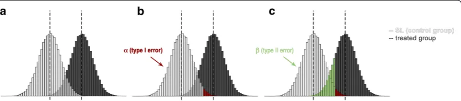
For calculation of the optimal test conditions, it is neces-sary to consider different error types as mathematical principals such as significance, power, and precision. In general, considering two concentrations (i.e. negative control and a test concentration >0), the associated ob-served effects are random values from two different
dis-tributions with concentration-specific mean values
(Fig. 2). If the test concentration has no effect, both dis-tributions and their means are identical. If the test con-centration has an effect, the associated mean is higher than the control group mean. The two distributions will in general show a certain overlap. If the test concentration in an experiment generates a result in the overlapping
range, it cannot safely be concluded from this result that the test concentration has a systematic effect greater than the control group. The observed value has a considerable probability also under control conditions (Fig. 2a). This means that two different errors may occur when assessing response data from control and test concentrations. A type I error occurs if an effect is interpreted as a concen-tration effect although it is an effect of the negative con-trol (Fig. 2b). The probability α of a type I error, also known as the level of significance (the pvalue), reflects the risk of the producer [36]. To keep the danger of a type I error small, the empirical significance level is computed in an actual statistical test procedure, and only if this probability is small (smaller than or equal to a pre-specified α), it is concluded that the test concentration had a systematically higher effect than the control condi-tion. The default value forαis 0.05 or 5 %. The other error that might occur in a statistical test is that a systematically higher response from the test concentration is not recog-nized as such, so that an existing effect remains un-detected (Fig. 2c). This is the type II error, the probability of which should also be restricted to a reasonable value. It reflects the risk of the consumer. A typical value for the
accepted type II error is β= 0.20 or 20 %. The
complementary probability of the type II error (= 1−β), which is the probability of detecting a systematic differ-ence between responses, is also known as the power or quality of the test. Consideration of the type II error seems to be much less common than considering the type I error [37], possibly because it demands an extra effort, but it is a constitutional component of experimental design. The probabilities of both errors depend (among others) on the group sizes involved. Increasing group sizes is the only way to reduce both error probabilities, and consequently, the crucial step in sample size planning is finding the min-imal group sizes for which the accepted sizes of both er-rors are not exceeded (Fig. 1b). The distributions shown in Figs. 2 and 1b get narrower with increasing group size, which decreases the zone in which values from both groups overlap so that observations can more safely be at-tributed to one of the groups.
The present proposal usesα= 5 % and β= 20 % as de-faults for accepted errors. Both values are not fixed but are frequently used in experimental design. They may be changed, but the user should be careful when relaxing these defaults, as too liberal requirements make the test procedure ineffectual. It should be kept in mind that with a β close to 50 %, the user will declare a truly
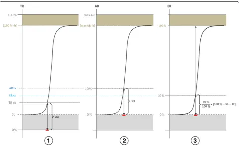
Fig. 3Risk types and their conversions:1total risk (TR),2added risk (AR),3extra risk (ER).IYimmunity,SLspontaneous lethality,xxtarget value (shown example = 10 %); converted values, max AR = [100−SL]; TR xx = xx = 10 %; AR xx = [SL + xx] = SL + 10 %; ER xx = xx/100 ·
existing effect with a probability of 50 % as not existing. This situation is equivalent to tossing a coin to obtain the test result. Obviously, a power analysis compliant to the individual target is a fundamental component in ex-perimental design [17].
Risk types
There are various ways of defining the response per-centage (the xx part in ECxx), differing by the way how
the spontaneous and the immune level are incorpo-rated. Three different common types of risks are con-sidered here. They differ in the way of how the concentration-related increase in the response is expressed. They will further be named as risk types. Each risk type (Fig. 3) has its own interpretation of xx and its specific value for ECxx, and it may also require
its own specific experimental design. The risk types used here are extended versions of the US Environmen-tal Protection Agency (EPA) definitions [38], whereas the extension consists in the additional consideration of immunity (IY) [28, 29]. Immunity describes the phenomenon that within a population, a subpopulation shows by chance no reaction at all. The EPA definitions result by setting IY = 0 %.
1. Total risk (TR): The total risk is the total response expressed as percentage of affected biological units among all treated units. Spontaneous lethality and immunity are ignored. Example: A desired xx = 10 % will force estimation of the concentration that generates an effect of 10 % (Fig.3(1)).
2. Added risk (AR): The reference frame is restricted below and above by spontaneous lethality and immunity. Only the response above the SL counts as an effect. Using AR, the total response associated with a target effect of size xx and a spontaneous lethality SL is xx + SL. Example: A desired AR of xx = 10 % and SL = 3.5 %, IY = 7 %, prompts estimating the concentration producing an effect of 10 % above the SL, equivalent to a total response of 13.5 %. The immunity parameter does generally not affect the ECxx value but restricts its possible maximum to
[100 %−SL−IY] (Fig.3(2)).
3. Extra risk (ER): The reference frame is the interval from SL to [100 %−IY]. Example: A desired ER with xx = 10 % and SL = 3.5 %, IY = 7 %, will force estimating the concentration which generates a total response of [SL + 0.01 · xx · (100 %−SL−IY)] = 3.5 % + 0.01 · 10 · (100 %−3.5 %−7 %) = 12.45 % (Fig.3(3)).
The total response associated with a target effect of xx and using ER as risk type is smaller than or equal to the
total response associated with the same xx, but with risk type AR.
Proposed software solution (toxtestD) for an optimal test design
To consider all our proposals, we implemented a pack-age with a set of functions in R code [39], which do ex-perimental design as outlined above in a user-friendly way. The R software is an open-source software. The package requires only a few inputs by the user. Sophisti-cated statistical understanding or modelling experiences are not necessary (though useful). Even though the concept is drafted for the fish embryo toxicity assay, it is possible to transfer the procedure in principle to all other toxicological questions, in which a continu-ous concentration equivalent generates a yes/no (bin-ary) response per single study object. The package
toxtestDshould already be consulted during the plan-ning phase of a test series. It contains the functions
spoD, setD, and doseD which cover identification of the spontaneous lethality, the estimation of the neces-sary number of test organisms, and a concentration design according to the user’s requirements. Examples for the application of all these functions are available after installation of the package by the command help (toxtestD) [40].
Determination of the spontaneous lethality byspoD
The first task when designing the experiment is calculat-ing the sample size for determincalculat-ing the SL. The neces-sary sample size depends on the required precision of the estimated SL. It should be recalled that because SL will be calculated from data containing random vari-ation, the resulting SL will also be a quantity with ran-dom error.
The function spoDoffers two services. In the planning process, the total number of individuals or eggs to test is calculated, together with a proposal for partitioning the total data set into subgroups in order to identify the amount of biological variation in the separated tests. The calculations will be done for the denoted rate and additionally for the worst case in the interval given for the predicted SL. The optimal number of biological units is calculated by using an exact binomial test with
α andβ as specified. The previous mentioned random
In the analysis process (initiated by setting analysis = TRUE), the spontaneous lethality together with its 95 % confidence interval and the biological variation are computed from the user’s data. Biological variation becomes visible when comparing spontaneous rates from several experiments under control conditions. A
χ2
test is applied to check whether these rates vary ac-cording to binomial variation under the hypothesis of the same true spontaneous rate for all experiments. A significant result signals the presence of biological variation between experiments. If present, its standard deviation is reported. It is recommended to determine the spontaneous lethality very early under separate test conditions.
Specifications by the user
Subprocess planning
n: The maximal number (integer) of test organisms, with which the laboratory is willing to cope. Limiting the number is necessary to avoid non-essential calculations and thereby save computing time. The programme will invite the user to increase the number if the number is not high enough to estimate the SL with the given preci-sion requirement.
SL.p: (optional SLmin, SLmax): To gain an optimal number of test objects for the determination of the true spontaneous lethality, the user needs at least a rough idea about the SL prior to test planning. This estimate is inserted in SL. It is possible to specify the SL either as single number or as an interval between 0 and 100 %. The maximum tolerated spontaneous lethality by OECD is 10 %. Datasets with higher SL should be discarded [9]. bio.sd.p (optional): The standard deviation of SL consists of normal random variation and a biological variation due to biological effects like season, daytime, or wellbeing. The default value of 2.008 % for bio.sd.p was determined from empirical data sets collected over 10 years by the Thünen Institute, Hamburg, Germany (U. Kammann and S. Schubert, personal communication) [41]. The value refers exclusively to dead eggs and lethal malformations (pursuant to the definition in DIN ENISO 15088) after 96 hpf in water in per cent [4, 9]. If not specified otherwise, this default will be used for determining the optimal number of partitions.
maxCI (optional): It is the maximally accepted absolute difference in per cent between mean SL and its confidence limits; default, 2.5 %.
print.result: If omitted, the result is written to a text file called ‘01_spontaneous lethality.txt’ in the calling directory. If a file name is given in double quotes, the result is written to that file. Nothing is written if FALSE is chosen.
Subprocess analysis
analysis: The default value is FALSE, indicating that the function does planning. To analyse the own dataset, choose analysis = TRUE.
SLdataset: This is the R data frame containing the experi-mental data. It needs two columns titled ‘n’ and ‘bearer’. In column n, the total number of observations of each single experimental run is listed. The column bearer comprises the number of organisms which are carriers (in the case of FET the counts of dead or lethal malformed eggs) within each single experimental run. Each row contains the outcome from one single experimental run.
Determination of the optimal number for each experimental run bysetD
The second task should be the calculation of the optimal number per experimental run. The proposed calcula-tions in setD involve a robustness consideration as it is done in the third task. We propose for every concentra-tion in the FET a sample size such that a test for a con-centration effect of size xx at the sought concon-centration ECxx would detect this effect with a high (pre-specified)
probability. Requiring a specified quality of the test leads to the necessary sample size per concentration. Two distributions will be estimated, one assuming SL as true response level, the other using SL + xx defined above (Fig. 1). The estimation of these two distribu-tions bases on binomial probability. The default of the distance is xx % in respect to a posterior target of ECxx.
Additionally the distance depends on the reference frame. In consequence, it is necessary to choose the convenient risk type (see section ‘Risk types’). The procedure in-creases the number of cases per concentration until the overlapping area of the two distributions corresponds to the specified levels of error types I and II (Fig. 1b).
Specifications by the user
nmax: Number (integer) of the maximum available number of organisms that can be tested in each treatment within an experimental run. The estimation of the optimal number will only start when this number is high enough to generate the response of at least one organism (nmax ·p> 1). If the chosen nmax is too small, a warning message is issued
SL.p: SL is calculated in per cent from own experimental data by the processspoD
then has [100 %−IY] as maximum. Please choose risk. type = 3 to include immunity in all calculations
risk.type: Please choose one of three risk types. Each type defines a specific reference frame for the concentration-response curve (for detailed information see the‘Risk types’section)
target.EC.p: The target response in per cent (e.g. 10 %, to calculate EC10). Note that the interpretation of
target.EC depends on the risk.type setting plot: There are three possibilities:
plot = FALSE: no plots
plot =‘single’: creates only one plot showing the two distr-ibutions under SL and under treated conditions with the optimal number of cases. Additionally, the real rates of error type one and two are given (see Fig. 1b). The special setting for risk.type is not included into this plot
plot =‘all’: In addition to the single plot, this option provides an estimation for all possibilities of target values. This gives an impression which possibilities of detection exist under the chosen conditions. This option may need a lot of computer capacity and time. It should not be activated in general.
alpha.p & beta.p: See explanations in‘Error types’section print.result: If omitted, the result is written to a text file called‘02_sample size.txt’in the calling directory. If a file name is given in double quotes, the result is written to that file. Nothing is written if FALSE is chosen
Allocating concentration points bydoseD
The third task, defining the concentration allocation for the main experiment, is guided by an idea of robustness similar to the second task. From a formal point of view, only as many concentration points as unknown parameters in the dose-response model are needed. It would however be unwise to involve only this minimum because it would not allow model checks. Concentration allocation needs at least a vague idea about position and scale of the concentration-response curve. Concentration-finding experiments, pilot studies, literature data, and similar sources are used to obtain these planning assumptions. Given an initial as-sumption, we propose the following concentration alloca-tion strategy: calculate EC10, EC50, EC90from the planning
assumptions, assuming a logistic concentration-response relation and involving SL and IY, if the selected risk type re-quires so. The control concentration of zero and these three concentrations plus target concentrations, given by the ECxx values of the experimenter’s interest, constitute
the concentration allocation pattern for the main experi-ment. Two-sided CIs with 95 and 99 % coverage probability will be calculated for the concentration-response curve. If more than four concentration points are chosen and there is an even number of free points, these will be allocated symmetrically around the chosen ECxx value. If two free
points are available, these are located at the limits of the 95 % CI. If an even number of 4 or more free points is available, these are allocated equidistantly in the 99 % CI. For an odd number of free points, 1 point is located at ECxx
and the others are allocated according to the rule for an even number. Note that the 1 of EC10, EC50, EC90can be
used twice as an experimental concentration, if the user’s target coincides with one of these. The strategy prefers low concentrations if several targets are specified by the user. This pattern is a robust strategy which fo-cuses on the main interest of finding ECxx but does
not rely too strongly on the planning assumptions. If previous experience suggests that the planning as-sumptions are realistic, concentrations could be allo-cated more closely around the presumed ECxx.
Specifications by the user
DP: The results from pre-tests must be given as a data frame with the columns‘name’,‘organisms’,‘death’,‘ con-centration’and‘unit’, which will be needed for the cal-culations of the dose scheme
immunity.p: immunity in per cent (see also settings of
spoD)
SL.p: SL is calculated in percent from the user’s experimental data by the functionspoD
target.EC.p: effect in %, which is of special interest. It is possible to denote more than one target in the same calculation. For example: if EC5 and EC10 are of
special interest, then target. EC =c (5,10) may be chosen, and the dose points will be allocated around both targets
nconc: number of different concentrations the user is willing to test in each cycle
text: text = TRUE adds extended information in the plot risk.type: Please choose one of three possible risk types.
Each type defines another reference frame for concentration-response curve and target estimation (for detailed information see the ‘Risk types’section). A plot for each risk type will be created separately print.result: If omitted, the result is written to a text file
called ‘03.dosestrategy.txt’in the calling directory. If a file name is given in double quotes, the result is written to that file. Nothing is written if FALSE is chosen.
Appendix
This appendix summarizes the main formulae that are proposed as part of the design procedure and are also incorporated in the R package.
The basic data in a concentration-response
experi-ment is the number n of examined objects and the
number r of responding objects. The empirical
re-sponse rate is the ratio p=r / n. It is frequently
This appendix, however, uses only rates, not percent-ages, for easier notation.
A CI is a way to express how precisely the response rate ptrue of the whole population is estimated by an
empirical rate. A confidence interval CI = (plow, phigh)
for an empirical rate is obtained from observed n and
rby [43]:
plow¼
r⋅F2ðn−rþ1Þ;2r;1−α=2
rþðn−rþ1Þ⋅F2ðn−rþ1Þ;2r;1−α=2
phigh¼ ðrþ1Þ⋅F2ðrþ1Þ;2ðn−rÞ;1−α=2 n−rþðrþ1Þ⋅F2ðrþ1Þ;2ðn−rÞ;1−α=2:
The F terms in both equations are the quantiles of the Fdistribution with degrees of freedom and associ-ated probability as given in the subscripts. The value of
α controls the coverage probability. The calculated
interval contains the value ptrue, which holds for the
whole population under study, with probability 1−α. This statement must be understood in a strategic sense: If the actual experiment is replicated many times and the CI is calculated for each replicate, then the popula-tion rateptruewill be contained in (1−α) · 100 % of the
calculated CIs.
The equation for the CI makes use of the fact that the
number r of responses has a binomial distribution,
which means that the probability of observing r
re-sponses among n examined subjects is as follows:
Prðr;n;ptrueÞ ¼ n
r ⋅p r
true⋅ð1−ptrueÞ
n−r:
Different concentrations xi of a substance generate their specificptrue(xi) values. A concentration-response (or dose-response) curve relates the probabilityptrueto
the dosex involved. This relation will always be a non-linear one, because the concentration or dose may be any value≥0 and the associated ptrue must lie in the
interval [0,1]. The present proposal uses the four-parameter logistic curve as concentration-response curve:
ptrueð Þ ¼x SLþ 1−SL−IY 1þe−ðaþb⋅xÞ:
The terms a and b in this equation control location and scale (slope) of the concentration-response relation. The values for these terms are estimated from I experi-ments with doses xi and numbers (ni, ri) of examined and responding objects by a maximum likelihood ap-proach by maximizing
logℓða;bjn;r;xÞ ¼X I
i
ni⋅logptrueða;bjxÞ
þðni−riÞ⋅log 1ð −ptrueða;bjxÞÞ:
The optimization is done iteratively by a Newton– Raphson approach. ECxxis obtained while using the
esti-mates for (a,b) by
ECxx¼−
1 b ln
1−SL−IY
xx−SL −1
þa
:
All calculations listed here are contained in the R package described.
Abbreviations
AR:Added risk; ASTM: ASTM International, known until 2001 as the American Society for Testing and Materials; BMD: Benchmark dose; DIN: German Institute for Standardization; EC: Effective concentration; ED: Effective dose; EPA: US Environmental Protection Agency; ER: Extra risk; FET: Fish embryo toxicity test; hpf: Hours post fertilization; IY: Immunity; LC: Lethal concentration; LD: Lethal dose; NOEC: No observed effect concentration; OECD: Organisation for Economic Co-operation and Development; REACH: Registration, Evaluation, Authorisation and Restriction of Chemicals; SL: Spontaneous lethality; TR: Total risk; VSD: Virtual safe dose.
Competing interests
The authors declare that they have no competing interests.
Authors’contributions
NK devised and realized the R package toxtestD and drafted the manuscript. SS has participated in the conception and design of the approach, performed all test runs (computer based as well as the FET), and has been involved in drafting the manuscript. WW has made substantial contributions to the conception and design of the R package and revised the manuscript critically for important intellectual content. All authors read and approved the final manuscript.
Acknowledgments
The authors thank Malte Damerau, Ulrike Kammann, Michael Haarich and Norbert Theobald for their thematic support. This study was incorporated into‘MERIT-MSFD: Methods for detection and assessment of risks for the marine ecosystem due to toxic contaminants in relation to implementation of the European Marine Strategy Framework Directive’. It was supported by a grant (grant number 10017012) from the German Federal Ministry of Transport and Digital Infrastructure (BMVI) and the German Maritime and Hydrographic Agency (BSH).
Author details
1Institute of Fisheries Ecology, Thünen Institute (TI), Palmaille 9, 22767
Hamburg, Germany.2Institute of Statistics, University of Bremen, Linzer Str. 4, 28334 Bremen, Germany.
Received: 8 October 2014 Accepted: 5 June 2015
References
1. r-project. http://cran.r-project.org/. 2015: Accessed: 18 Dec 2014. 2. Keddig N, Wosniok W. toxtestD package manual. http://cran.r-project.org/
web/packages/toxtestD/toxtestD.pdf. 2014.
3. Lammer E, Carr GJ, Wendler K, Rawlings JM, Belanger SE, Braunbeck T. Is the fish embryo toxicity test (FET) with the zebrafish (Danio rerio) a potential alternative for the fish acute toxicity test? Comparative Biochemistry and Physiology Part C: Toxicology & Pharmacology. 2009;149(2):196–209. http://dx.doi.org/10.1016/j.cbpc.2008.11.006.
5. Keiter S, Peddinghaus S, Feiler U, von der Goltz B, Hafner C, Ho NY, et al. A novel joint research project using zebrafish (Danio rerio) to identify specific toxicity and molecular modes of action of sediment-bound pollutants.
J Soils Sediments. 2010;10:714–7. doi:10.1007/s11368-010-0221-7. 6. Research Centre for Toxic Compounds in the Environment. http://
www.recetox.muni.cz/index-en.php?pg=research-and-development– analyses-and-services–ecotoxicology. 2014: Accessed: 01 Apr 2014.
7. Fraunhofer-Gesellschaft. http://www.ime.fraunhofer.de/de/ geschaeftsfelderAE/Verbleib_und_Wirkung_Agrochemikalien/ Erweiterte_Standardtests.html#tabpanel-5. 2014: Accessed: 01 Apr 2014. 8. Microtest Laboratories. http://www.microtestlabs.com. 2014: Accessed:
1 Apr 2014.
9. Organisation for Economic Co-operation and Development. OECD guidelines for the testing of chemicals - fish embryo acute toxicity (FET) test. 2013;236 (adopted 26 July 2013).
10. Hutchinson TH, Solbe J, Kloepper-Sams PJ. Analysis of the ecetoc aquatic toxicity (EAT) database III—comparative toxicity of chemical substances to different life stages of aquatic organisms. Chemosphere. 1998;36(1):129–42. http://dx.doi.org/10.1016/S0045-6535(97)10025-X.
11. Crump KS. Calculation of benchmark doses from continuous data. Risk Anal. 1995;15(1):79–89.
12. European Chemicals Agency. Guidance on information requirements and chemical safety assessment Chapter R.10: Characterisation of dose [concentration]-response for environment. 2008. http://echa.europa.eu/ documents/10162/13632/information_requirements_r10_en.pdf. 13. Van Der Hoeven N. How to measure no effect. Part III: statistical aspects of
NOEC, ECx and NEC estimates. Environmetrics. 1997;8(3):255–61. doi:10.1002/(SICI)1099-095X(199705)8:3<255::AID-ENV246>3.0.CO;2-P. 14. Chapman PM, Caldwell RS, Chapman PF. A warning: NOECs are
inappropriate for regulatory use. Environ Toxicol Chem. 1996;15:77–9. 15. Crane M, Newman MC. What level of effect is a no observed effect? Environ
Toxicol Chem. 2000;19(2):516–9. doi:10.1002/etc.5620190234.
16. Moore DRJ, Caux P-Y. Estimating low toxic effects. Environ Toxicol Chem. 1997;16(4):794–801. doi:10.1002/etc.5620160425.
17. Warne MSJ, van Dam R. NOEC and LOEC data should no longer be generated or used. Australas J Ecotoxicol. 2008;14:1–5.
18. Landis WG, Chapman PM. Well past time to stop using NOELs and LOELs. Integr Environ Assess Manag. 2011;7(4):vi–vii. doi:10.1002/ieam.249. 19. Grasso P. Essentials of pathology for toxicologists. Taylor & Francis Inc.,
London, New York 2002.
20. van Ewijk PH, Hoekstra JA. Calculation of the EC50 and its confidence interval when subtoxic stimulus is present. Ecotoxicol Environ Saf. 1993;25(1):25–32. http://dx.doi.org/10.1006/eesa.1993.1003. 21. European Union. Directive 2008/56/EG - Marine strategy framework
directive. In: Union OJotE, editor.2008.
22. Federal Institute for Occupational Safety and Health, (BAuA). Hazardous substances ordinance (Gefahrstoffverordnung–GefStoffV). 2010; updated. 2013. 23. Institute for Health and Consumer Protection. Technical guidance
document on risk assessment. 2003.
24. European Union. Regulation (EC) No 1907/2006 of the European Parliament and of the council. 2006.
25. Fraysse B, Mons R, Garric J. Development of a zebrafish 4-day embryo-larval bioassay to assess toxicity of chemicals. Ecotoxicology and Environmental Safety. 2006;63(2):253–67. http://dx.doi.org/10.1016/j.ecoenv.2004.10.015. 26. Piegorsch WW, Xiong H, Bhattacharya RN, Lin L. Benchmark dose analysis
via nonparametric regression modeling. Risk analysis: an official publication of the Society for Risk Analysis. 2013:1–17. doi:10.1111/risa.12066. 27. Kammann U, Vobach M, Wosniok W, Schäffer A, Telscher A. Acute toxicity of
353-nonylphenol and its metabolites for zebrafish embryos. Environ Sci Pollut Res. 2009;16(2):227–31.
28. Ratkowsky DA, Reedy TJ. Choosing near-linear parameters in the four-parameter logistic model for radioligand and related assays. Biometrics. 1986;42(3):575–82. doi:10.2307/2531207.
29. DeLean A, Munson PJ, Rodbard D. Simultaneous analysis of families of sigmoidal curves: application to bioassay, radioligand assay, and physiological dose-response curves. Am J Physiol Gastrointest Liver Physiol. 1978;235(2):G97–G102.
30. Carlsson G, Patring J, Kreuger J, Norrgren L, Oskarsson A. Toxicity of 15 veterinary pharmaceuticals in zebrafish (Danio rerio) embryo. Aquat Toxicol. 2013;126(0):30–41. http://dx.doi.org/10.1016/j.aquatox.2012.10.008.
31. Hayes JP. The positive approach to negative results in toxicology studies. Ecotoxicol Environ Saf. 1987;14(1):73–7. http://dx.doi.org/10.1016/0147-6513(87)90085-6.
32. Wedekind C, von Siebenthal B, Gingold R. The weaker points of fish acute toxicity tests and how tests on embryos can solve some issues. Environ Pollut. 2007;148(2):385–9. http://dx.doi.org/10.1016/j.envpol.2006.11.022. 33. Kent M, Buchner C, Barton C, Tanguay R. Toxicity of chlorine to zebrafish
embryos. Dis Aquat Org. 2014;107(3):235–40. doi:10.3354/dao02683. 34. European Union. Directive 2010/63/EU of the European Parliament and of
the council on the protection of animals used for scientific purposes. In: Union OJotE, editor.2010. p. 33–79.
35. Braunbeck T, Böttcher M, Hollert H, Kosmehl T, Lammer E, Leist E, et al. Towards an alternative for the acute fish LC (50) test in chemical assessment: the fish embryo toxicity test goes multi-species—an update. Altex. 2004;22(2):87–102.
36. Gad SC. Statistics and experimental design for toxicologists and pharmacologists. Taylor & Francis Group, LLC, Boca Raton, London, New York, Singapore; 2005.
37. Fairweather PG. Statistical power and design requirements for environmental monitoring. Mar Freshw Res. 1991;42(5):555–67. 38. United States Environmental Protection Agency (U.S. EPA). EPA’s approach
for assessing the risks associated with chronic exposure to carcinogens—Integrated Risk Information System (IRIS): http:// www.epa.gov/iris/carcino.htm. 1992: Accessed 10 Sept 2014. 39. R Core Team. R: A language and environment for statistical computing.
R Foundation for Statistical Computing. 2014;Vienna, Austria. http://www. R-project.org/
40. Keddig N, Wosniok W. toxtestD package—experimental design for binary toxicity tests (with examples). 2014. http://cran.r-project.org/web/packages/ toxtestD/index.html.
41. Kammann U, Vobach M, Wosniok W. Toxic effects of brominated indoles and phenols on zebrafish embryos. Arch Environ Contam Toxicol. 2006;51(1):97–102. doi:10.1007/s00244-005-0152-2.
42. Dinse G, An EM. Algorithm for fitting a four-parameter logistic model to binary dose-response data. JABES. 2011;16(2):221–32. doi:10.1007/s13253-010-0045-3. 43. Johnson NL, Kotz S. Distributions in statistics: discrete distributions. Wiley
Interscience; New York; Brisbane 1969.
Submit your manuscript to a
journal and benefi t from:
7 Convenient online submission
7 Rigorous peer review
7 Immediate publication on acceptance
7 Open access: articles freely available online
7 High visibility within the fi eld
7 Retaining the copyright to your article