Estimation of the threat of IEMI to complex electronic systems

(1)

Radio Science

Estimation of the threat of IEMI to complex electronic systems

R. Kanyou Nana1, S. Korte2, S. Dickmann1, H. Garbe2, and F. Sabath3

1_{Helmut-Schmidt-Universität/Universität der Bundeswehr Hamburg, Germany} 2_{Leibniz-Universität Hannover, Germany}

3_{Wehrwissenschaftliches Institut f¨ur Schutztechnologien, Munster, Germany}

Abstract. The threat of ultra wideband (UWB) sources is in-teresting for military issues. This paper summarizes informa-tion concerning the voltages generated from some commer-cially available UWB generator systems and their produced electromagnetic fields. The paper focuses on the coupling of UWB fields into electronic equipment and discusses possi-ble modeling and measurement techniques to estimate such a threat for modern ships. An evaluation procedure for the determination of the induced voltage at the input of an elec-tronic component is presented. This method is based on the computation of the internal electric field and the measure-ments on a test network, which is similar to the structure of the steering control cabling. It allows the estimation of the potential threat for the ship’s electronic equipment due to the exposal to UWB emitting sources.

1 Introduction

In complex systems like ships or aircrafts many tasks vital to the function of the system are executed by electronic equip-ment. Earlier research from Ianoz and Wipf (2000) as well as Radasky (2006) has shown, that there are frequency ranges in many of these systems, where disturbances in the system will be observed if an external electromagnetic field exceeds a certain limit. This induced effect in an electronic equipment is commonly known as IEMI (intentional electromagnetic interference). In order to understand the threats to modern ships, it is necessary to define the electromagnetic environ-ment, that can cause operational problems for exposed ship systems. With respect to criminal purposes e.g. terrorism, it is useful to consider an intentional electromagnetic envi-ronment (IEME) created by UWB generator systems. For

Correspondence to: R. Kanyou Nana ([email protected])

this type of threat, a produced pulse typically has frequency components over a wide spectral range. Due to the fact that many systems have resonances that create significant suscep-tibilities to particular frequencies as mentioned above, it is possible that ship systems are affected by the voltages and currents caused by incident UWB fields. This can cause dis-turbances or failures in these systems which could lead to severe problems.

The structure of this paper is as follows: the modeling of the problem is presented in Sect. 2. Starting with the volt-ages from some commercially available UWB generator sys-tems, a brief overview concerning the derivation of the inci-dent fields is given in Sect. 3. After that, in Sect. 4, mod-eling and measurement techniques for the description of the different coupling mechanisms into the considered system, here the chassis of the steering control and an Ethernet test network, are discussed. Aspects for the estimation of UWB threats for marine equipment, like the computation of the in-ternal fields and the induced disturbance voltage at the input of an electronic component, are in the focus of Sect. 5.

2 Modeling of the problem

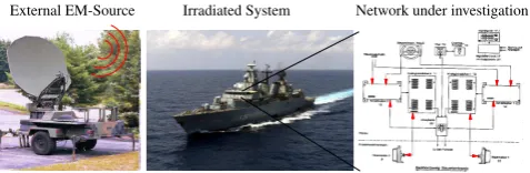
The problem faced here is illustrated in Fig. 1. It shows a frigate irradiated by a transient electromagnetic field of an

Manuscript prepared for Adv. Radio Sci.

with version 2.3 of the LA_{TEX class copernicus.cls.}

Date: 12 December 2008

Estimation of the threat of IEMI to complex electronic systems

R. Kanyou Nana1_{, S. Korte}2_{, S. Dickmann}1_{, H. Garbe}2_{, and F. Sabath}3 1_{Helmut - Schmidt - Universität / Universität der Bundeswehr Hamburg} 2_{Leibniz - Universität Hannover}

3_{Wehrwissenschaftliches Institut f¨ur Schutztechnologien, Munster}

Abstract.The threat of ultra wideband (UWB) sources is in-teresting for military issues. This paper summarizes informa-tion concerning the voltages generated from some commer-cially available UWB generator systems and their produced electromagnetic fields. The paper focuses on the coupling of UWB fields into electronic equipment and discusses possi-ble modeling and measurement techniques to estimate such a threat for modern ships. An evaluation procedure for the determination of the induced voltage at the input of an elec-tronic component is presented. This method is based on the computation of the internal electric field and the measure-ments on a test network, which is similar to the structure of the steering control cabling. It allows the estimation of the potential threat for the ship’s electronic equipment due to the exposal to UWB emitting sources.

1 Introduction

In complex systems like ships or aircrafts many tasks vital to the function of the system are executed by electronic equip-ment. Earlier research from Ianoz and Wipf (2000) as well as Radasky (2006) has shown, that there are frequency ranges in many of these systems, where disturbances in the system will be observed if an external electromagnetic field exceeds a certain limit. This induced effect in an electronic equip-ment is commonly known as IEMI (intentional electromag-netic interference). In order to understand the threats to mo-dern ships, it is necessary to define the electromagnetic en-vironment, that can cause operational problems for exposed ship systems. With respect to criminal purposes e.g. terror-ism, it is useful to consider an intentional electromagnetic en-vironment (IEME) created by UWB generator systems. For this type of threat, a produced pulse typically has frequency

Correspondence to:R. Kanyou Nana ([email protected])

components over a wide spectral range. Due to the fact that many systems have resonances that create significant suscep-tibilities to particular frequencies as mentioned above, it is possible that ship systems are affected by the voltages and currents caused by incident UWB fields. This can cause dis-turbances or failures in these systems which could lead to severe problems.

The structure of this paper is as follows: the modeling of the problem is presented in section 2. Starting with the voltages from some commercially available UWB generator systems, a brief overview concerning the derivation of the incident fields is given in section 3. After that, in section 4, mode-ling and measurement techniques for the description of the different coupling mechanisms into the considered system, here the chassis of the steering control and an Ethernet test network, are discussed. Aspects for the estimation of UWB threats for marine equipment, like the computation of the in-ternal fields and the induced disturbance voltage at the input of an electronic component, are in the focus of section 5.

2 Modeling of the problem

The problem faced here is illustrated in fig1. It shows a

fri-External EM-Source Irradiated System Network under investigation

Fig. 1. Geometry of the system, which is irradiated by a transient electromagnetic field of an external interfering source

gate irradiated by a transient electromagnetic field of an

ex-Fig. 1. Geometry of the system, which is irradiated by a transient

electromagnetic field of an external interfering source.

(2)

250 R. Kanyou Nana et al.: IEMI to complex systems

ternal UWB interfering source. The determination of the coupling into an internal network of this system is a typical EMC problem which can be devided into three parts: source, coupling paths and sink as shown in fig.2.

Interfering source Coupling structures Device

Source Coupling paths Sink

Fig. 2.Coupling interference as a typical EMC problem

The determination of the radiated electric far-field E1(jω)

is suitable for the characterisation of the external interfering source. Therewith the needed incident electromagnetic field can be calculated:

E(jω) =E1(jω)r1

r; H(jω) = E(jω)

Z0

=r1·E1(jω) r·Z0

, (1) whereZ0represents the free space wave impedance.E1(jω)

stands for the (known) radiated electric far-field evaluated at a distancer1from the interfering source and (E(jω), H(jω))

are the incident electromagnetic field, which must be deter-mined at the distancerfrom the interfering source (placed directly in front of the investigated system, here the ship). The coupling paths are generally modelled with system trans-fer functions. Since most devices connected to the exam-ined network have metallic enclosures, it can be assumed that electromagnetic disturbances predominantly couple into the electronic devices through the transmission lines. There-fore the input impedance of the device adequately describes it as the sink. A detailed partitioning of the initial problem is shown in fig.3.

Fig. 3.Detailed description of the coupling interference

This approach is based on the knowledge of the radiated elec-tric far-field in time domaine1(t), which makes it possible

to determine the spectra of the incident electromagnetic field E(jω), H(jω)by using the FFT (Fast Fourier Transform) and the formulas in (1). Because the electric as well as the magnetic part of the field contribute to the overall coupling in the definition domain of the system transfer functions, the coupling of the external electromagnetic field into the elec-tronics can be described in the frequency domain by sepa-rated system transfer functionsFEU(jω)andFHU(jω). They

establish the interrelationship between the external electro-magnetic fieldE(jω),H(jω)and the fraction of voltages at the terminals of the electronic componentsUE(jω),UH(jω)

in the investigated network. The product of both fractions of the fieldE(jω)andH(jω)with the corresponding system transfer functionFEU(jω)andFHU(jω)yields the fractional

system responsesUE(jω)andUH(jω). The superposition of

these intermediate results leads to the system response in the frequency domainU(jω), which next can be used to obtain the system response in the time domain u(t) by using the IFFT (Inverse Fast Fourier Transform).

SinceFEU(jω)andFHU(jω)strongly depend on the

geom-etry of the system, a structure modification in the system (i.e. the dimensions of the apertures or the load impedances) requires a complete new computation. It has been shown in Kanyou Nana (2008), that FEU(jω) ratherFHU(jω)are

made up of contributions from several coupling paths of elec-tromagnetic fields, which are represented by different (el-ementary) transfer functions. In the scope of this problem the coupling through apertures predominates. Thus, for the determination of the coupled disturbance voltages, first the internal electromagnetic fieldEint(jω),Hint(jω)in a close

vicinity of the network should be evaluated. This field is then used to excite the network (model based on the equivalent generators along the cables and the transmission lines of the network). Consequently the initial system transfer functions ( fig. 3) can be decomposed in field and coupling transfer functions (fig.4), which implies that a structure modification in the system solely requires a re-evaluation of the affected transfer functions. The disadvantage of this method is that

Fig. 4.Decomposition of the system transfer functions illustrated in fig.3in field (FEE(jω),FHH(jω)) and coupling transfer functions (FEU(jω),FHU(jω))

not only two but at least four transfer functions are neces-sary to perform a complete analysis of the problem. For net-work problems in which the electromagnetic field is consid-ered as primary source, it has been proven in Tesche, Ianov and Karlsson (1996) that the effect of the magnetic field can be expressed by the electric field. This typical solution form of network problems is known asAgrawal method. For the present case, this means that only the knowledge of the inter-nal electric fieldEint(jω)is required for the computation of

the disturbance voltageU(jω). Thus, the number of transfer functions can be reduced to the half as presented in fig.5.

Fig. 2. Coupling interference as a typical EMC problem.

The determination of the radiated electric far-field E1(jω)

is suitable for the characterisation of the external interfering source. Therewith the needed incident electromagnetic field can be calculated:

E(jω) =E1(jω)

r1

r; H(jω) = E(jω)

Z0 =

r1·E1(jω)

r·Z0 , (1)

whereZ0represents the free space wave impedance.E1(jω)

stands for the (known) radiated electric far-field evaluated at a distancer1from the interfering source and (E(jω), H(jω))

are the incident electromagnetic field, which must be deter-mined at the distance rfrom the interfering source (placed directly in front of the investigated system, here the ship). The coupling paths are generally modelled with system trans-fer functions. Since most devices connected to the exam-ined network have metallic enclosures, it can be assumed that electromagnetic disturbances predominantly couple into the electronic devices through the transmission lines. There-fore the input impedance of the device adequately describes it as the sink. A detailed partitioning of the initial problem is shown in fig.3.

This approach is based on the knowledge of the radiated elec-tric far-field in time domaine1(t), which makes it possible

to determine the spectra of the incident electromagnetic field E(jω), H(jω)by using the FFT (Fast Fourier Transform) and the formulas in (1). Because the electric as well as the magnetic part of the field contribute to the overall coupling in the definition domain of the system transfer functions, the coupling of the external electromagnetic field into the elec-tronics can be described in the frequency domain by sepa-rated system transfer functionsFEU(jω)andFHU(jω). They

establish the interrelationship between the external electro-magnetic fieldE(jω),H(jω)and the fraction of voltages at the terminals of the electronic componentsUE(jω),UH(jω)

in the investigated network. The product of both fractions of the fieldE(jω)andH(jω)with the corresponding system transfer functionFEU(jω)andFHU(jω)yields the fractional

system responsesUE(jω)andUH(jω). The superposition of

these intermediate results leads to the system response in the frequency domainU(jω), which next can be used to obtain the system response in the time domain u(t)by using the IFFT (Inverse Fast Fourier Transform).

SinceFEU(jω)andFHU(jω)strongly depend on the

geom-etry of the system, a structure modification in the system (i.e. the dimensions of the apertures or the load impedances) requires a complete new computation. It has been shown in Kanyou Nana (2008), thatFEU(jω)rather FHU(jω)are

made up of contributions from several coupling paths of elec-tromagnetic fields, which are represented by different (el-ementary) transfer functions. In the scope of this problem the coupling through apertures predominates. Thus, for the determination of the coupled disturbance voltages, first the internal electromagnetic fieldEint(jω),Hint(jω)in a close

vicinity of the network should be evaluated. This field is then used to excite the network (model based on the equivalent generators along the cables and the transmission lines of the network). Consequently the initial system transfer functions ( fig. 3) can be decomposed in field and coupling transfer functions (fig.4), which implies that a structure modification in the system solely requires a re-evaluation of the affected transfer functions. The disadvantage of this method is that

Fig. 4.Decomposition of the system transfer functions illustrated in fig.3in field (FEE(jω),FHH(jω)) and coupling transfer functions (FEU(jω),FHU(jω))

not only two but at least four transfer functions are neces-sary to perform a complete analysis of the problem. For net-work problems in which the electromagnetic field is consid-ered as primary source, it has been proven in Tesche, Ianov and Karlsson (1996) that the effect of the magnetic field can be expressed by the electric field. This typical solution form of network problems is known asAgrawal method. For the present case, this means that only the knowledge of the inter-nal electric fieldEint(jω)is required for the computation of

the disturbance voltageU(jω). Thus, the number of transfer functions can be reduced to the half as presented in fig.5.

Fig. 3. Detailed description of the coupling interference.

external UWB interfering source. The determination of the coupling into an internal network of this system is a typical EMC problem which can be devided into three parts: source, coupling paths and sink as shown in Fig. 2.

The determination of the radiated electric far-fieldE1(jω) is suitable for the characterisation of the external interfering source. Therewith the needed incident electromagnetic field can be calculated:

E(jω)=E1(jω)

r1

r; H (jω)= E(jω)

Z0

=r1·E1(jω)

r·Z0

, (1) whereZ0represents the free space wave impedance.E1(jω) stands for the (known) radiated electric far-field evaluated at a distancer1from the interfering source and (E(jω), H (jω)) are the incident electromagnetic field, which must be deter-mined at the distancer from the interfering source (placed directly in front of the investigated system, here the ship). The coupling paths are generally modelled with system trans-fer functions. Since most devices connected to the exam-ined network have metallic enclosures, it can be assumed that electromagnetic disturbances predominantly couple into the electronic devices through the transmission lines. There-fore the input impedance of the device adequately describes it as the sink. A detailed partitioning of the initial problem is shown in Fig. 3.

This approach is based on the knowledge of the radiated electric far-field in time domaine1(t ), which makes it pos-sible to determine the spectra of the incident electromag-netic field E(jω), H (jω) by using the FFT (Fast Fourier Transform) and the formulas in (1). Because the electric as well as the magnetic part of the field contribute to the overall coupling in the definition domain of the system trans-fer functions, the coupling of the external electromagnetic field into the electronics can be described in the frequency domain by separated system transfer functionsFEU(jω)and

FHU(jω). They establish the interrelationship between the external electromagnetic field E(jω), H (jω) and the frac-tion of voltages at the terminals of the electronic components

UE(jω), UH(jω)in the investigated network. The product

The determination of the radiated electric far-field E1(jω) is suitable for the characterisation of the external interfering source. Therewith the needed incident electromagnetic field can be calculated:

E(jω) =E1(jω)

r1

r; H(jω) = E(jω)

Z0 =

r1·E1(jω)

r·Z0 , (1) whereZ0represents the free space wave impedance.E1(jω) stands for the (known) radiated electric far-field evaluated at a distancer1from the interfering source and (E(jω), H(jω)) are the incident electromagnetic field, which must be deter-mined at the distancerfrom the interfering source (placed directly in front of the investigated system, here the ship). The coupling paths are generally modelled with system trans-fer functions. Since most devices connected to the exam-ined network have metallic enclosures, it can be assumed that electromagnetic disturbances predominantly couple into the electronic devices through the transmission lines. There-fore the input impedance of the device adequately describes it as the sink. A detailed partitioning of the initial problem is shown in fig.3.

This approach is based on the knowledge of the radiated elec-tric far-field in time domaine1(t), which makes it possible to determine the spectra of the incident electromagnetic field

E(jω), H(jω) by using the FFT (Fast Fourier Transform) and the formulas in (1). Because the electric as well as the magnetic part of the field contribute to the overall coupling in the definition domain of the system transfer functions, the coupling of the external electromagnetic field into the elec-tronics can be described in the frequency domain by sepa-rated system transfer functionsFEU(jω)andFHU(jω). They

establish the interrelationship between the external electro-magnetic fieldE(jω),H(jω)and the fraction of voltages at the terminals of the electronic componentsUE(jω),UH(jω) in the investigated network. The product of both fractions of the fieldE(jω)andH(jω)with the corresponding system transfer functionFEU(jω)andFHU(jω)yields the fractional system responsesUE(jω)andUH(jω). The superposition of these intermediate results leads to the system response in the frequency domainU(jω), which next can be used to obtain the system response in the time domainu(t) by using the IFFT (Inverse Fast Fourier Transform).

SinceFEU(jω)andFHU(jω)strongly depend on the geom-etry of the system, a structure modification in the system (i.e. the dimensions of the apertures or the load impedances) requires a complete new computation. It has been shown in Kanyou Nana (2008), thatFEU(jω)rather FHU(jω) are made up of contributions from several coupling paths of elec-tromagnetic fields, which are represented by different (el-ementary) transfer functions. In the scope of this problem the coupling through apertures predominates. Thus, for the determination of the coupled disturbance voltages, first the internal electromagnetic fieldEint(jω),Hint(jω)in a close vicinity of the network should be evaluated. This field is then used to excite the network (model based on the equivalent generators along the cables and the transmission lines of the network). Consequently the initial system transfer functions ( fig. 3) can be decomposed in field and coupling transfer functions (fig.4), which implies that a structure modification in the system solely requires a re-evaluation of the affected transfer functions. The disadvantage of this method is that

Fig. 4.Decomposition of the system transfer functions illustrated in fig.3in field (FEE(jω),FHH(jω)) and coupling transfer functions (FEU(jω),FHU(jω))

not only two but at least four transfer functions are neces-sary to perform a complete analysis of the problem. For net-work problems in which the electromagnetic field is consid-ered as primary source, it has been proven in Tesche, Ianov and Karlsson (1996) that the effect of the magnetic field can be expressed by the electric field. This typical solution form of network problems is known asAgrawal method. For the present case, this means that only the knowledge of the inter-nal electric fieldEint(jω)is required for the computation of the disturbance voltageU(jω). Thus, the number of transfer functions can be reduced to the half as presented in fig.5.

Fig. 4. Decomposition of the system transfer functions illustrated in

Fig. 3 in field (FEE(jω),FHH(jω)) and coupling transfer functions

(FEU(jω),FHU(jω)).

of both fractions of the fieldE(jω)andH (jω)with the cor-responding system transfer function FEU(jω)andFHU(jω) yields the fractional system responsesUE(jω)andUH(jω). The superposition of these intermediate results leads to the system response in the frequency domainU (jω), which next can be used to obtain the system response in the time domain

u(t )by using the IFFT (Inverse Fast Fourier Transform). Since FEU(jω)andFHU(jω) strongly depend on the ge-ometry of the system, a structure modification in the system (i.e. the dimensions of the apertures or the load impedances) requires a complete new computation. It has been shown in Kanyou Nana (2008), thatFEU(jω)ratherFHU(jω)are made up of contributions from several coupling paths of electro-magnetic fields, which are represented by different (elemen-tary) transfer functions. In the scope of this problem the cou-pling through apertures predominates. Thus, for the determi-nation of the coupled disturbance voltages, first the internal electromagnetic fieldEint(jω),Hint(jω)in a close vicinity of the network should be evaluated. This field is then used to excite the network (model based on the equivalent generators along the cables and the transmission lines of the network). Consequently the initial system transfer functions (Fig. 3) can be decomposed in field and coupling transfer functions (Fig. 4), which implies that a structure modification in the system solely requires a re-evaluation of the affected transfer functions.

The disadvantage of this method is that not only two but at least four transfer functions are necessary to perform a complete analysis of the problem. For network problems in which the electromagnetic field is considered as primary source, it has been proven in Tesche, Ianov and Karlsson (1996) that the effect of the magnetic field can be expressed by the electric field. This typical solution form of network problems is known as Agrawal method. For the present case, this means that only the knowledge of the internal electric fieldEint(jω)is required for the computation of the distur-bance voltageU (jω). Thus, the number of transfer functions can be reduced to the half as presented in Fig. 5.

(3)

R. Kanyou Nana et al.: IEMI to complex systems 251

Fig. 5. Simplification of the transfer functions shown in fig.4by making use of the Agrawal method

3 Characterisation of the interfering source

Voltages from commercial UWB pulse generators can be generally approximated with the analytical functions shown in table1. Next it will be proven that the knowledge of the

Table 1.Analytical description of the voltages from some commer-cial UWB pulse generator systems

generator voltage enables a description of the radiated elec-tric field and after that the derivation of an analytical expres-sion for the electric far-field. Here the signal forms shown in fig.6are considered, which correspond to the graphical representations of the pulses in table1: the half sine pulse, the unipolar double exponential pulse as well as the full sine pulse. The radiation of these signals can be realised with the

Fig. 6.Voltages from some commercial UWB generator systems

following types of antennas:

– the TEM Horn antenna (Half and Full sine pulses), and

– the reflector antenna Type IRA (unipolar double expo-nential pulse).

Because antennas generally have a derivative behaviour, the radiated electric far-field is proportional to the time derivative of the generator voltage:

ei(t)∼

dui(t)

dt . (2)

The normalization of dui(t)

dt with its maximum value

consequently results in the normalized electric far-field

ei(t)/eimax. For the above-mentioned generator voltages, fig. 7 illustrates the resulting electric field. A use of

Fig. 7. Estimated normalized electric far-fields generated from some commercial UWB generator systems

the FFT on ei(t)/eimax yields the normalized spectrum

Ei(jω)/eimax, the magnitude of which is shown in fig. 8. The needed spectrumEi(jω)results from the multiplication

Fig. 8. Magnitude of normalized spectra of the estimated electric far-fields

of the normalized spectrum with the maximum field value

eimaxthat depends on the type of antenna.

4 Characterisation of the coupling structures

For the characterisation of the coupling effects of electro-magnetic field pulses into complex systems, the field trans-fer functionFEE(jω)as well as the coupling transfer func-tionFEU(jω)were introduced. A field transfer function is a function that transforms a field from one position (i.e. the external incident field) into another field on another position (i.e. the field inside the chassis of the steering control next to the network). A coupling transfer function is a function that converts a field from one position (i.e. the field inside the chassis of the steering control next to the network) into a voltage on a precise point of the network (i.e. the induced voltage at the device’s input). In the following, these transfer functions will be quantified in order to describe the existing coupling structures of the investigated system.

4.1 Modeling of the ship

To compute the field transfer function FEE(jω), numerical simulations were performed using the 3D-FDTD based code PAM-CEM/FD. Due to the size and the complexity of the ship, we used a simplified model, in which only the bridge (which contents the chassis of the steering control) was taken into account, because it can be regarded as effectively iso-lated from the rest of the ship. The bridge is modeled as

Fig. 5. Simplification of the transfer functions shown in Fig. 4 by

making use of the Agrawal method.

Table 1. Analytical description of the voltages from some

commer-cial UWB pulse generator systems.

generator voltage enables a description of the radiated elec-tric field and after that the derivation of an analytical expres-sion for the electric far-field. Here the signal forms shown in fig. 6are considered, which correspond to the graphical representations of the pulses in table1: the half sine pulse, the unipolar double exponential pulse as well as the full sine pulse. The radiation of these signals can be realised with the

ei(t)∼

dui(t)

dt . (2)

dt with its maximum value consequently results in the normalized electric far-field

ei(t)/eimax. For the above-mentioned generator voltages,

fig. 7 illustrates the resulting electric field. A use of

Ei(jω)/eimax, the magnitude of which is shown in fig.8.

The needed spectrumEi(jω)results from the multiplication

of the normalized spectrum with the maximum field value eimaxthat depends on the type of antenna.

For the characterisation of the coupling effects of electro-magnetic field pulses into complex systems, the field trans-fer functionFEE(jω)as well as the coupling transfer

func-tionFEU(jω)were introduced. A field transfer function is

a function that transforms a field from one position (i.e. the external incident field) into another field on another position (i.e. the field inside the chassis of the steering control next to the network). A coupling transfer function is a function that converts a field from one position (i.e. the field inside the chassis of the steering control next to the network) into a voltage on a precise point of the network (i.e. the induced voltage at the device’s input). In the following, these transfer functions will be quantified in order to describe the existing coupling structures of the investigated system.

To compute the field transfer functionFEE(jω), numerical

simulations were performed using the 3D-FDTD based code PAM-CEM/FD. Due to the size and the complexity of the ship, we used a simplified model, in which only the bridge (which contents the chassis of the steering control) was taken into account, because it can be regarded as effectively iso-lated from the rest of the ship. The bridge is modeled as

3 Characterisation of the interfering source

Voltages from commercial UWB pulse generators can be generally approximated with the analytical functions shown in Table 1.

Next it will be proven that the knowledge of the genera-tor voltage enables a description of the radiated electric field and after that the derivation of an analytical expression for the electric far-field. Here the signal forms shown in Fig. 6 are considered, which correspond to the graphical represen-tations of the pulses in Table 1: the half sine pulse, the unipo-lar double exponential pulse as well as the full sine pulse. The radiation of these signals can be realised with the fol-lowing types of antennas:

– the TEM Horn antenna (Half and Full sine pulses), and – the reflector antenna Type IRA (unipolar double

expo-nential pulse).

ei(t )∼ dui(t )

dt . (2)

The normalization of dui(t )

dt with its maximum value

consequently results in the normalized electric far-field

ei(t )/eimax. For the above-mentioned generator voltages, Fig. 7 illustrates the resulting electric field. A use of the FFT onei(t )/eimaxyields the normalized spectrumEi(jω)/eimax, the magnitude of which is shown in Fig. 8. The needed spec-trumEi(jω)results from the multiplication of the normalized spectrum with the maximum field valueeimax that depends on the type of antenna.

generator voltage enables a description of the radiated elec-tric field and after that the derivation of an analytical expres-sion for the electric far-field. Here the signal forms shown in fig. 6are considered, which correspond to the graphical representations of the pulses in table1: the half sine pulse, the unipolar double exponential pulse as well as the full sine pulse. The radiation of these signals can be realised with the

ei(t)∼ dui(t)

dt . (2)

Ei(jω)/eimax, the magnitude of which is shown in fig. 8.

func-tion FEU(jω)were introduced. A field transfer function is

Fig. 6. Voltages from some commercial UWB generator systems.

generator voltage enables a description of the radiated elec-tric field and after that the derivation of an analytical expres-sion for the electric far-field. Here the signal forms shown in fig.6 are considered, which correspond to the graphical representations of the pulses in table1: the half sine pulse, the unipolar double exponential pulse as well as the full sine pulse. The radiation of these signals can be realised with the

ei(t)∼dui(t)

dt . (2)

Ei(jω)/eimax, the magnitude of which is shown in fig. 8.

Fig. 7. Estimated normalized electric far-fields generated from some commercial UWB generator systems.

4 Characterisation of the coupling structures

For the characterisation of the coupling effects of electro-magnetic field pulses into complex systems, the field transfer functionFEE(jω) as well as the coupling transfer function

FEU(jω)were introduced. A field transfer function is a func-tion that transforms a field from one posifunc-tion (i.e. the exter-nal incident field) into another field on another position (i.e. the field inside the chassis of the steering control next to the network). A coupling transfer function is a function that con-verts a field from one position (i.e. the field inside the chassis of the steering control next to the network) into a voltage on a precise point of the network (i.e. the induced voltage at the device’s input). In the following, these transfer functions will be quantified in order to describe the existing coupling structures of the investigated system.

4.1 Modeling of the ship

To compute the field transfer function FEE(jω), numerical simulations were performed using the 3D-FDTD based code PAM-CEM/FD. Due to the size and the complexity of the ship, we used a simplified model, in which only the bridge (which contents the chassis of the steering control) was taken into account, because it can be regarded as effectively iso-lated from the rest of the ship. The bridge is modeled as a metal cavity containing just the relevant metallic objects (Fig. 9). One of these objects is the steering control unit.

While modeling the chassis of the steering control, its ba-sic structure and the internal big metallic objects have been taken into account. Smaller structures like complicated har-nesses were been neglected. Since the coupling field in the chassis is generated through the slots, it was necessary to dis-cretize the smallest dimension of each implemented slot with at least two patches. The used PAM-CEM/FD model of the chassis is depicted in Fig. 10.

(4)

generator voltage enables a description of the radiated elec-tric field and after that the derivation of an analytical expres-sion for the electric far-field. Here the signal forms shown in fig.6 are considered, which correspond to the graphical representations of the pulses in table1: the half sine pulse, the unipolar double exponential pulse as well as the full sine pulse. The radiation of these signals can be realised with the

ei(t)∼ dui(t)

dt . (2)

Ei(jω)/eimax, the magnitude of which is shown in fig.8.

To compute the field transfer function FEE(jω), numerical

Fig. 8. Magnitude of normalized spectra of the estimated electric

far-fields.

4 R. Kanyou Nana et al.: IEMI to complex systems

a metal cavity containing just the relevant metallic objects

(Fig.

9 ). One of these objects is the steering control unit.

Fig. 9.A view of the simplified bridge model

While modeling the chassis of the steering control, its basic

structure and the internal big metallic objects have been taken

into account. Smaller structures like complicated harnesses

were been neglected. Since the coupling field in the chassis

is generated through the slots, it was necessary to discretize

the smallest dimension of each implemented slot with at least

two patches. The used PAM-CEM/FD model of the chassis

is depicted in fig.

10 .

Fig. 10.PAM-CEM/FD model of the chassis of the steering control

After modeling the different parts of the structure, it was

nec-essary to define the type of the excitation of the system. The

whole system was illuminated by a vertical and horizontal

polarised electromagnetic field, respectively. Then the

nor-malisation of the computed electric field inside the bridge

with respect to the incident field yields to the simulated field

transfer function.

Measurements were performed to validate the numerical

modeling. A simplified block diagram of the measurement

points and the instrumentation is shown in fig.

11 . The

mea-Fig. 11.Block diagram of measurement points and instrumentation for validation of the simplified bridge model

surement for the evaluation

F

EE

(j

ω

)

was performed in two

steps. First a reference measurement was done without the

ship and second the measurement was carried out on the

ship, where all measuring instruments were placed inside the

bridge except the transmitting antenna. The ratio between

both measurement results yields to the desired transfer

func-tion. For point

P

1

the magnitude of

F

EE

(j

ω

)

in the

simula-tions and measurements, in the case of a vertical polarized

field, are compared in fig.

12 . From a EMC point of view,

100 200 300 400 500 600 700 800 900 1000 10−3

10−2 10−1 100 101

f/MHz

|F

EE

|

Measurement Simulation

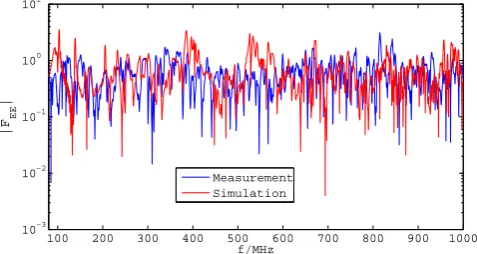
Fig. 12.Comparison of calculated and measured field transfer func-tion at the pointP1inside the chassis of the steering control

both results agree quite well. Thus, the presented model can

be used to estimate the field in the chassis of the steering

control.

4.2 Ethernet test network

The coupling transfer function

F

EU

(j

ω

)

was determined with

measurements of an ethernet cable (type: cat 5) with an

overall length of 5 m and terminated with

100 Ω

load

re-Fig. 9. A view of the simplified bridge model.

After modeling the different parts of the structure, it was necessary to define the type of the excitation of the system. The whole system was illuminated by a vertical and hori-zontal polarised electromagnetic field, respectively. Then the normalisation of the computed electric field inside the bridge with respect to the incident field yields to the simulated field transfer function.

Measurements were performed to validate the numerical modeling. A simplified block diagram of the measurement points and the instrumentation is shown in Fig. 11. The measurement for the evaluationFEE(jω)was performed in two steps. First a reference measurement was done without the ship and second the measurement was carried out on the ship, where all measuring instruments were placed inside the bridge except the transmitting antenna. The ratio between both measurement results yields to the desired transfer func-tion. For point P1 the magnitude ofFEE(jω)in the simula-tions and measurements, in the case of a vertical polarized field, are compared in Fig. 12. From a EMC point of view, both results agree quite well. Thus, the presented model can be used to estimate the field in the chassis of the steering control.

4.2 Ethernet test network

The coupling transfer functionFEU(jω)was determined with measurements of an ethernet cable (type: cat 5) with an

a metal cavity containing just the relevant metallic objects (Fig.9). One of these objects is the steering control unit.

While modeling the chassis of the steering control, its basic structure and the internal big metallic objects have been taken into account. Smaller structures like complicated harnesses were been neglected. Since the coupling field in the chassis is generated through the slots, it was necessary to discretize the smallest dimension of each implemented slot with at least two patches. The used PAM-CEM/FD model of the chassis is depicted in fig.10.

After modeling the different parts of the structure, it was nec-essary to define the type of the excitation of the system. The whole system was illuminated by a vertical and horizontal

polarised electromagnetic field, respectively. Then the nor-malisation of the computed electric field inside the bridge with respect to the incident field yields to the simulated field transfer function.

Measurements were performed to validate the numerical modeling. A simplified block diagram of the measurement points and the instrumentation is shown in fig.11. The

surement for the evaluationFEE(jω)was performed in two steps. First a reference measurement was done without the ship and second the measurement was carried out on the ship, where all measuring instruments were placed inside the bridge except the transmitting antenna. The ratio between both measurement results yields to the desired transfer func-tion. For pointP1the magnitude ofFEE(jω)in the simula-tions and measurements, in the case of a vertical polarized field, are compared in fig.12. From a EMC point of view,

100 200 300 400 500 600 700 800 900 1000

10−3 10−2

10−1 100 101

f/MHz

|F

EE

|

Fig. 12.Comparison of calculated and measured field transfer

func-tion at the pointP1inside the chassis of the steering control

both results agree quite well. Thus, the presented model can be used to estimate the field in the chassis of the steering control.

4.2 Ethernet test network

The coupling transfer functionFEU(jω)was determined with measurements of an ethernet cable (type: cat 5) with an overall length of 5 m and terminated with100 Ωload re-Fig. 10. PAM-CEM/FD model of the chassis of the steering control.

4 R. Kanyou Nana et al.: IEMI to complex systems

a metal cavity containing just the relevant metallic objects

(Fig.

9 ). One of these objects is the steering control unit.

While modeling the chassis of the steering control, its basic

structure and the internal big metallic objects have been taken

into account. Smaller structures like complicated harnesses

were been neglected. Since the coupling field in the chassis

is generated through the slots, it was necessary to discretize

the smallest dimension of each implemented slot with at least

two patches. The used PAM-CEM/FD model of the chassis

is depicted in fig.

10 .

After modeling the different parts of the structure, it was

nec-essary to define the type of the excitation of the system. The

whole system was illuminated by a vertical and horizontal

polarised electromagnetic field, respectively. Then the

nor-malisation of the computed electric field inside the bridge

with respect to the incident field yields to the simulated field

transfer function.

Measurements were performed to validate the numerical

modeling. A simplified block diagram of the measurement

points and the instrumentation is shown in fig.

11 . The

surement for the evaluation

F

EE

(j

ω

)

was performed in two

steps. First a reference measurement was done without the

ship and second the measurement was carried out on the

ship, where all measuring instruments were placed inside the

bridge except the transmitting antenna. The ratio between

both measurement results yields to the desired transfer

func-tion. For point

P

1

the magnitude of

F

EE

(j

ω

)

in the

simula-tions and measurements, in the case of a vertical polarized

field, are compared in fig.

12 . From a EMC point of view,

100 200 300 400 500 600 700 800 900 1000

10−3 10−2 10−1 100 101

f/MHz

|F

EE

|

both results agree quite well. Thus, the presented model can

be used to estimate the field in the chassis of the steering

control.

4.2 Ethernet test network

The coupling transfer function

F

EU

(j

ω

)

was determined with

measurements of an ethernet cable (type: cat 5) with an

overall length of 5 m and terminated with

100 Ω

load

re-Fig. 11. Block diagram of measurement points and instrumentation

for validation of the simplified bridge model.

overall length of 5 m and terminated with 100load resis-tance. Its magnitude for different coupling lengths is pre-sented in Fig. 13. As can be seen, the magnitude ofFEU(jω) depends strongly on the coupling length and has frequency components only from 17 MHz to 200 MHz. This frequency range contains the first resonance frequency of the used ca-ble (20 MHz), which can be calculated using the following formula (εr=2.25, µr=1):

f = c

2l√εrµr

. (3)

5 Estimation of the induced voltages

With respect to the above-mentioned UWB antenna types, the peak value of the electric field, which can be achieved at a distance of about 1 km without exagger-ation, are in the order of 50 V/m for a TEM-horn (30 cm×30 cm×30 cm, umax=50 kV) and 34 V/m for an IRA (∅: 90 cm, umax=9 kV). Such levels of fields should therefore be considered in order to assess the induced volt-age on a 100 load resistance at the end of the ethernet cable. Multiplying these maximum field values with the cor-responding normalized electric field from Fig. 8, the incident

(5)

a metal cavity containing just the relevant metallic objects

(Fig.

9 ). One of these objects is the steering control unit.

While modeling the chassis of the steering control, its basic

structure and the internal big metallic objects have been taken

into account. Smaller structures like complicated harnesses

were been neglected. Since the coupling field in the chassis

is generated through the slots, it was necessary to discretize

the smallest dimension of each implemented slot with at least

two patches. The used PAM-CEM/FD model of the chassis

is depicted in fig.

10 .

After modeling the different parts of the structure, it was

nec-essary to define the type of the excitation of the system. The

whole system was illuminated by a vertical and horizontal

polarised electromagnetic field, respectively. Then the

nor-malisation of the computed electric field inside the bridge

with respect to the incident field yields to the simulated field

transfer function.

Measurements were performed to validate the numerical

modeling. A simplified block diagram of the measurement

points and the instrumentation is shown in fig.

11 . The

surement for the evaluation

F

EE

(j

ω

)

was performed in two

steps. First a reference measurement was done without the

ship and second the measurement was carried out on the

ship, where all measuring instruments were placed inside the

bridge except the transmitting antenna. The ratio between

both measurement results yields to the desired transfer

func-tion. For point

P

1

the magnitude of

F

EE

(j

ω

)

in the

simula-tions and measurements, in the case of a vertical polarized

field, are compared in fig.

12 . From a EMC point of view,

100 200 300 400 500 600 700 800 900 1000 10−3

10−2 10−1 100 101

f/MHz

|F

EE

|

both results agree quite well. Thus, the presented model can

be used to estimate the field in the chassis of the steering

control.

4.2 Ethernet test network

The coupling transfer function

F

EU

(j

ω

)

was determined with

measurements of an ethernet cable (type: cat 5) with an

overall length of 5 m and terminated with

100 Ω

load

re-Fig. 12. Comparison of calculated and measured field transfer

func-tion at the point P1inside the chassis of the steering control.

100 101 102 103

0 0.01 0.02 0.03

f / MHz |F EU

| / V/(V/m)

51 cm coupling length 29 cm coupling length 11 cm coupling length

Fig. 13. Measured coupling transfer function of a 100terminated ethernet cable for 51 cm, 29 cm and 11 cm coupling lengths.

electric field in the frequency domain can be estimated. A multiplication of this field with both the field transfer func-tion and the coupling transfer funcfunc-tion, and followed by IFFT, leads to the desired induced voltage. The results are presented in Fig. 14. As can be seen, induced voltages up to 0.06–0.1 V appear at the entry of a sensitive electronic equip-ment, which can lead to functional disturbances for some electronics.

6 Conclusions

With regard to commercially available UWB generator sys-tems, a methodology for the derivation of the incident elec-tric fields has been presented. With the help of these fields and by using both the field and the coupling transfer func-tions of the investigated system, a first estimation of the in-duced disturbance voltage at the entry of ship’s electronics has been done. These results can be used to estimate the threat of such a system under IEMI.

sistance. Its magnitude for different coupling lengths is pre-sented in fig.13. As can be seen, the magnitude ofFEU(jω)

100 101 102 103

0 0.01 0.02 0.03

f / MHz

|FEU

| / V/(V/m)

51 cm Koppellänge 29 cm Koppellänge 11 cm Koppellänge

Fig. 13.Measured coupling transfer function of a100 Ωterminated ethernet cable for 51 cm, 29 cm and 11 cm coupling lengths

depends strongly on the coupling length and has frequency components only from 17 MHz to 200 MHz. This frequency range contains the first resonance frequency of the used ca-ble (20 MHz), which can be calculated using the following formula (εr= 2.25, µr= 1):

f = c

2l√εrµr . (3)

5 Estimation of the induced voltages

With respect to the above-mentioned UWB antenna types, the peak value of the electric field, which can be achieved at a distance of about 1 km without exaggeration, are in the or-der of50 V/mfor a TEM-horn (30 cm x 30 cm x 30 cm,

umax= 50 kV) and 34 V/m for an IRA (∅: 90 cm,

umax= 9 kV). Such levels of fields should therefore be

con-sidered in order to assess the induced voltage on a100 Ω

load resistance at the end of the ethernet cable. Multiplying these maximum field values with the corresponding normal-ized electric field from fig.8, the incident electric field in the frequency domain can be estimated. A multiplication of this field with both the field transfer function and the coupling transfer function, and followed by IFFT, leads to the desired induced voltage. The results are presented in fig.14.

As can be seen, induced voltages up to 0.06 - 0.1 V appear at the entry of a sensitive electronic equipment, which can lead to functional disturbances for some electronics.

6 Conclusions

With regard to commercially available UWB generator sys-tems, a methodology for the derivation of the incident elec-tric fields has been presented. With the help of these fields

Half sine Double exponential Full sine

Fig. 14.Estimated induced voltage on a100 Ωload resistance for an 5 m length ethernet cable (coupling length: 51 cm)

and by using both the field and the coupling transfer func-tions of the investigated system, a first estimation of the in-duced disturbance voltage at the entry of ship’s electronics has been done. These results can be used to estimate the threat of such a system under IEMI.

Acknowledgement. This work has been financed by the Bundesamt f¨ur Wehrtechnik und Beschaffung. The authors would like to thank P. Dietz of the Einsatzflottille 2 (German Navy) for his support.

References

Ianoz, M. and Wipf, H.: Modeling and Simulation Methods to As-sess EM Terrorism Effects, Asia-Pacific Conference on Environ-mental Electromagnetics CEEM, Shanghai, China, 2000. Radasky, W. A.: The Threat of Intentional Electromagnetic

Interfer-ence (IEMI) to Wired and Wireless Systems, 17th International Zurich Symposium on Electromagnetic Compatibility, Zurich, Switzerland, pp.110-163, 2006.

Kanyou Nana, R., Dickmann, S., and Sabath, F.: Electromagnetic field vulnerability of complex systems – an application of EM topology, Advances in Radio Science, 6, 1-5, 2008.

Tesche, F. M., Ianov, M. V., and Karlsson T.: EMC Analysis Meth-ods and Computational Models, ISBN 0-471-15573-X, John Wi-ley & Sons, Inc., New York, 1996.

Camp, M.: Empfindlichkeit elektronischer Schaltungen gegen tran-siente elektromagnetische Feldimpulse, ISBN 3-8322-3504-3, Shaker Verlag, Dissertation, Universit¨at Hannover, 2004. Sonnemann, F.: Susceptibility Investigations of High-Power

EM-Fields on electronic systems, International Symposium and technical Exhibition on electromagnetic Compatibility, Zurich, Switzerland, 2003.

Baum, C. E.: Electromagnetic Topology: A formal approach to the analysis and design of complex electronic systems, Proc. Zurich EMC Symp., 209-214, 1982.

Paul, C. R.: Analysis of Multiconductor Transmission Lines, ISBN 0-471-02080-X, John Wiley & Sons, Includes bibliographical references and index, New York, 1994.

Giri, D. V.: Radiation of impulse-like waveforms with illustra-tive applications, Ultrawideband and Ultrashort Impulse Signals, Sevastopol, Ukraine, pp.19-22 September, 2004.

IEEE Std. 299: IEEE Standard Method for Measuring the Effective-ness of Electromagnetic Shielding Enclosures, IEEE Inc., 345 East 47 Street, New York, NY 10017, 1997.

Fig. 14. Estimated induced voltage on a 100load resistance for an 5 m length ethernet cable (coupling length: 51 cm).

Acknowledgement. This work has been financed by the Bundesamt

f¨ur Wehrtechnik und Beschaffung. The authors would like to thank P. Dietz of the Einsatzflottille 2 (German Navy) for his support.

References

Ianoz, M. and Wipf, H.: Modeling and Simulation Methods to As-sess EM Terrorism Effects, Asia-Pacific Conference on Environ-mental Electromagnetics CEEM, Shanghai, China, 2000. Radasky, W. A.: The Threat of Intentional Electromagnetic

Interfer-ence (IEMI) to Wired and Wireless Systems, 17th International Zurich Symposium on Electromagnetic Compatibility, Zurich, Switzerland, 110–163, 2006.

Kanyou Nana, R., Dickmann, S., and Sabath, F.: Electromagnetic field vulnerability of complex systems – an application of EM topology, Adv. Radio Sci., 6, 273–277, 2008,

http://www.adv-radio-sci.net/6/273/2008/.

Tesche, F. M., Ianov, M. V., and Karlsson T.: EMC Analysis Meth-ods and Computational Models, ISBN: 0-471-15573-X, John Wiley & Sons, Inc., New York, USA, 1996.

Camp, M.: Empfindlichkeit elektronischer Schaltungen gegen tran-siente elektromagnetische Feldimpulse, ISBN 3-8322-3504-3, Shaker Verlag, Dissertation, Universit¨at Hannover, 2004. Sonnemann, F.: Susceptibility Investigations of High-Power

EM-Fields on electronic systems, International Symposium and technical Exhibition on electromagnetic Compatibility, Zurich, Switzerland, 2003.

Baum, C. E.: Electromagnetic Topology: A formal approach to the analysis and design of complex electronic systems, Proc. Zurich EMC Symp., 209–214, 1982.

Paul, C. R.: Analysis of Multiconductor Transmission Lines, ISBN 0-471-02080-X, John Wiley & Sons, Includes bibliographical references and index, New York, USA, 1994.

Giri, D. V.: Radiation of impulse-like waveforms with illustra-tive applications, Ultrawideband and Ultrashort Impulse Signals, Sevastopol, Ukraine, 19–22, September 2004.

IEEE Std. 299: IEEE Standard Method for Measuring the Effective-ness of Electromagnetic Shielding Enclosures, IEEE Inc., 345 East 47 Street, New York, NY 10017, USA, 1997.