R E S E A R C H
Open Access
Clustering algorithm for audio signals
based on the sequential Psim matrix and
Tabu Search
Wenfa Li
1, Gongming Wang
2*and Ke Li
1Abstract
Audio signals are a type of high-dimensional data, and their clustering is critical. However, distance calculation failures, inefficient index trees, and cluster overlaps, derived from the equidistance, redundant attribute, and sparsity, respectively, seriously affect the clustering performance. To solve these problems, an audio-signal clustering
algorithm based on the sequential Psim matrix and Tabu Search is proposed. First, the audio signal similarity is calculated with the Psim function, which avoids the equidistance. The data is then organized using a sequential Psim matrix, which improves the indexing performance. The initial clusters are then generated with differential truncation and refined using the Tabu Search, which eliminates cluster overlap. Finally, the K-Medoids algorithm is used to refine the cluster. This algorithm is compared to the K-Medoids and spectral clustering algorithms using UCI waveform datasets. The experimental results indicate that the proposed algorithm can obtain better Macro-F1 and Micro-F1 values with fewer iterations.
Keywords:Audio signal clustering, Sequential Psim matrix, Tabu Search, Heuristic search, K-Medoids, Spectral clustering
1 Introduction
Audio signal clustering forms the basis for speech recog-nition, audio synthesis, audio retrieval, etc. Audio signals are considered as high-dimensional data, with dimen-sionalities of more than 20 [1]. Their clustering is under-taken based on this consideration and solving the problems in high-dimensional data clustering, in this re-gard, is highly beneficial.
There are three types of clustering algorithms for high-dimensional data: attribute reduction [2], subspace clus-tering [3], and co-clusclus-tering [4]. The first method reduces the data dimensionality with attribute conversion or re-duction and then, performs clustering. The effect of this method is heavily dependent on the degree of dimension reduction; if it is considerable, useful information may be lost, and if it is less, clustering cannot be done effectively. The second method divides the original space into several different subspaces and searches for cluster in the sub-space. When the dimensionality is high and the accuracy
requirement rigorous, the number of subspaces rapidly in-creases. Thus, searching for a cluster in a subspace be-comes a bottleneck and may lead to failure [5]. The third method implements clustering iteratively with respect to the content and feature alternately. The clustering result is adjusted as per the semantic relationship between the theme and characteristic, realizing a balance between data and attribute clustering. This method has two stages, resulting in a high time complexity. In addition to the above three methods, clustering algorithms for high-dimensional data includes hierarchical clustering [6], par-allel clustering [7], knowledge-driven clustering [8], etc. However, these methods also have similar problems.
Equidistance, the redundant attribute, and sparsity are the fundamental factors affecting the clustering perform-ance of high-dimensional data [9]. Equidistperform-ance renders the distance between any two points in a high-dimensional space approximately equal, leading to a failure in the clus-tering algorithm, based on the distance. The redundant
at-tribute increases the dimensionality of the
high-dimensional data and the complexity of the index structure, decreasing the efficiency of building and retrieving the index structure. Sparsity enables uniform data distribution,
* Correspondence:[email protected]
2Institute of Biophysics, Chinese Academy of Sciences, No. 15 Datun Road, Beijing, China
Full list of author information is available at the end of the article
and some clusters may overlap with each other, affecting the clustering precision.
It is reported that some dimensional components of the high-dimensional data are non-related noise that hide the real distance, resulting in equidistance. The Psim function can find and eliminate noise in all the di-mensions [10]. The Tabu Search [11] is a heuristic global search algorithm. All the possible existent clusters are combinatorically optimized using the Tabu Search such that a non-overlap cluster is selected.
To solve the clustering problems owing to equidis-tance, the redundant attribute, and sparsity, an efficient audio signal clustering algorithm is proposed, by integra-tion with the Psim matrix and Tabu Search. First, for all the points in the high-dimensional space, the Psim values between them and the corresponding location numbers are stored in a Psim matrix. Next, a sequential Psim matrix is generated by sorting the elements in each row of the Psim matrix. Further, the initial clusters are generated with differential truncation and refined with the Tabu Search. Finally, the initial clusters are iteratively refined with the K-Medoids algorithm, until all the clus-ter medoids are stable.
2 Related works 2.1 Psim matrix
Traditional similarity measurement methods (e.g., the Eu-clidean distance, Jaccard coefficient [12], and Pearson co-efficient [12]) fail in high-dimensional space because in these methods, equidistance is a common phenomenon in high-dimensional space; hence, the calculated distance is not the real distance. To solve this problem, the Hsim function [13] was proposed; however, the relative differ-ence and noise distribution were not considered. The Gsim function [14] was also proposed and the relative dif-ferences of the properties in different dimensions were an-alyzed, but the weight discrepancy was ignored. The proposed Close function [15] can reduce the influence of components in certain dimensions, whose variances are larger; however, the relative difference was not considered and it would be affected by noise. The Esim [16] function was proposed by improving the Hsim and Close functions and considering the influence of the property on the simi-larity. In every dimension, the Esim component has a positive correlation. All the dimensions are divided into normal and noisy. In a noisy dimension, noise is the main ingredient. When it is similar and larger than the signal, in a normal dimension, Esim is invalid. The secondary meas-urement method [17] is used to calculate the similarity by considering the property distribution, space distance, etc. However, the noise distribution and weight are not taken into account. In addition, its formula is complicated and the calculation is slow. In high-dimensional space, a large difference exists in certain dimensionalities [10], even
though the data is similar. This difference occupies a large portion of the similarity calculation; hence, all the calcula-tion results are similar. Therefore, the Psim funccalcula-tion [10] was proposed to diminish the influence of noise on the similarity data; experimental results indicate that this method is suitable.
When using the Psim function to measure the similar-ity, the data component in every dimension must be sorted and the value range divided into several intervals. The similarity betweenX and Yin the j-th dimension is added to the Psim function, if and only if, their data components are in the same interval.
In an n-dimensional space, the Psim value between X
andYis as follow:
PsimðX;YÞ ¼ X j∈Ds Xð;YÞ
1−jXj−Yjj lj−uj
DsðX;YÞ
j j
n
whereXjand Yj are the data components ofX and Yin the j-th dimension. Ds(X,Y) is a subscript set of Xjand Yj, which are in the same interval [uj,lj], and |Ds(X,Y)| is the number of elements in Ds(X,Y). The above is the outline of the Psim function; a detailed introduction can be found in [10].
Data organization is critical in a clustering algorithm. In the traditional method, the data space is separated using an index tree and mapped onto the index-tree nodes. The commonly used index trees are the R tree [18], cR tree [19], VP tree [20], M tree [21], SA tree [22], etc. The partitioning of the data space is the foundation for building an index tree, but its complexity increases with the increase in dimensionality. Thus, it is difficult to build index trees for high-dimensional data. In addition, the retrieval efficiency of the index tree falls sharply with the increase in dimensionality. The retrieval function works effectively, when the dimensionality is less than 16; however, it weakens rapidly, for dimension-alities greater than 16, even down to the level of a linear search [23]. A sequential Psim matrix is used to solve this problem. First, all the Psim values between points, S1, S2, ⋯, SM, are calculated to build a Psim matrix,
PsimMat, with a size,M×M. PsimMat(i,t) is composed of three properties: i, t, and Psim(Si,St). Next, the se-quential Psim matrix, SortPsimMat, is generated by sort-ing the elements in every row of PsimMat in the descending order of the Psim value. The elements in the i-th row represent the similarities between Si and the other points. From left to right, the Psim values grad-ually diminish, indicating a decrease in the similarity. It can be seen that the sequential Psim matrix is not af-fected by the dimensionality and can represent the simi-larity distribution of all the points. Therefore, it is suitable for high-dimensional data clustering.
2.2 Differential truncation
The elements in every row of SortPsimMat are regarded as a sequence,A, whose length isM. The sequential Psim differential matrix, DeltaPsimMat, is generated with a dif-ferential operation on the sequence,A. The size of DeltaP-simMat is M× (M−1). The elements in the i-th row of SortPsimMat represent the similarities betweenSiand the
other points. Several points corresponding to the frontier elements in this row, from the left, would form a cluster centered atSibecause the similarity between the elements
inside the cluster is higher than that of those outside. Thus, the similarity differences between the elements in-side the cluster are lesser than that of the others. Assum-ing that the cluster centered atSihaspielements, the left
pi−1elements in thei-th row of DeltaPsimMat are lesser
than the differential threshold,ΔAmax. Thus, a reasonable
ΔAmax is set up and all the elements that are less than
ΔAmaxin thei-th row of DeltaPsimMat are found to form
a cluster centered atSi.
2.3 Tabu Search
After differential truncation, the intersection of some of the clusters may not be null. Thus, the overlapping ele-ments should be eliminated by refinement. The clusters that are to be refined are called the imminent-refining cluster sets, and the initial values are the clusters after differential truncation. The clusters that have been re-fined are called the rere-fined cluster sets and their initial values are null. The refinement of the cluster is an itera-tive process. Considering the average Psim of the
re-mainder elements in the i-th row of SortPsimMat, after
differential truncation, as the similarity of a cluster cen-tered atSi, the operation in every iteration is as follows:
First, the similarity of every cluster is calculated. Next, the cluster with the highest similarity is added into the refined cluster set and the element in the other cluster is deleted, if it is in the selected cluster. However, there is a problem. After deleting the overlapping elements, the similarity of the cluster in the imminent-refining cluster set may be greater than that of the selected cluster. To solve this problem, Tabu Search is used for refinement.
Tabu Search is an expansion of the neighborhood search, a global optimum algorithm [11], and is mainly used for combinatorial optimization. A roundabout search can be avoided using the Tabu rule and aspiration criterion, for improving the global search efficiency. This method can accept an inferior solution and has a strong “climbing”ability; it has a higher probability of obtaining a global optimal solution.
The main process of Tabu Search is as follows: Initially, a random initial solution is regarded as the current solu-tion, and several neighboring solutions are considered as the candidate solutions. Further, if the objective function value of a certain candidate solution meets the aspiration
criterion, the current solution is replaced by this candidate solution and added to the Tabu list. Else, the best choice of a non-Tabu object is considered as the new current so-lution. In addition, the corresponding solution must be added into the Tabu list [24]. The above steps are re-peated, until the terminate criterion is satisfied.
In order to use Tabu Search for refining the cluster, an appropriate Tabu object, Tabu list, aspiration criterion, and terminate criterion are required. The Tabu objects are the elements in the refined cluster set and are saved into the Tabu list to prevent the Tabu Search from falling into the local optimum. The Tabu length is set as the number of clusters after differential truncation. In every iteration process, the selected cluster is considered as the Tabu ob-ject. After eliminating the overlapping elements, the cluster, whose similarity is higher than that of the previously se-lected cluster, is considered as the better cluster and it re-places the previously selected cluster. The previously selected cluster is removed from the Tabu list and added into the imminent-refining cluster set. The above“ eliminat-ing the overlappeliminat-ing elements—searching for a better clus-ter”process is repeated, until a better cluster can no longer be found. Then, the previously selected cluster is consid-ered as the optimal cluster of this iteration. The search for the better cluster of the next iteration then commences, until the imminent-refining cluster set is null.
3 Clustering algorithm 3.1 Problem description
The dataset of M audio signals with a length, n, is con-sidered as the point set, S= {S1,S2,⋯,SM}, of n
-dimen-sional space, where Si= {Si1,⋯,Sij,⋯,Sin}, i= 1, 2, ⋯,
M,j= 1, 2,⋯,n, andSijare thej-th property ofSi.
The goal is to search for sets,C1,C2,⋯,CK, that meet
the following two requirements:
1. C1∪C2∪ ∪CK=S
2. Cv∩Cw=φ, for any 1≤v≠w≤K.
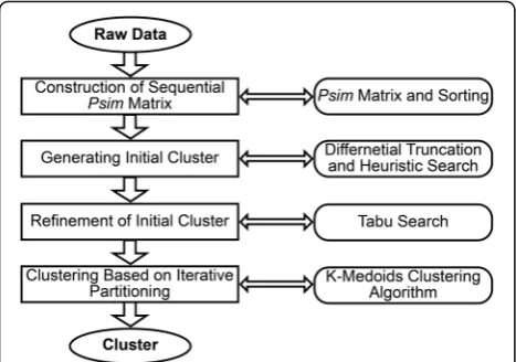
3.2 Framework of the clustering algorithm
The proposed clustering algorithm has four steps, as shown in Fig. 1. First, the sequential Psim matrix is built to represent the similarity between the points in the set, S. Next, the initial cluster is generated by integration with the differential truncation and heuristic search. Fur-ther, the initial cluster is refined with Tabu Search. Fi-nally, the expected cluster is generated by clustering, based on the K-Medoids.
3.3 Clustering algorithm procedure
3.3.1 Construction of a sequential Psim matrix
are sorted with quicksort to obtain the sequential Psim matrix, SortPsimMat. The above is a brief introduction; the detailed procedure can be found in [25].
3.3.2 Initial cluster generation
First, the Laplacian matrix, L, is generated by PsimMat, and its eigenvalue distribution is used to determine the number of expected clusters [26]. Next, the differential threshold,ΔAmax, is initialized. LetCmaxbe the maximal
time for searching the cluster set. The upper bound of Cmax is the combinatorial number, CKM, where K is the
number of clusters. Searching CKM times is
time-consuming because the magnitude of CKM is M!. In
addition, the K expected clusters maybe not found by
searchingCKM times. Thus,Cmaxis set toCmax=Mand a
heuristic search is implemented. Finally, the collision list of the clusters, TBLC, is set to null and i=1. Then, the
initial cluster can be generated with the following steps.
Step 1: The elements in thei-th row of DeltaPsimMat are visited from left to right, until thepi-th element is greater than the differential threshold,ΔAmax, for the first time.
Step 2: The points corresponding to the leftpi‐1 elements in thei-th row of SortPsimMat are used to construct a cluster,CiT, centered atSi.
Step 3: Ifi<M, theni=i+1; go to Step 1; else,c=1. Step 4:Kclusters,Ci1
T;CiT1;⋯;CiKT, are selected fromM
clusters,C1T;C2T;⋯;CMT, to ensure that the set
composed ofKcenters of the selected cluster are not in the Tabu list,TBLC.
Step 5: If the union of K clusters is equal to the set,
S, then the set, Ci¼ C0i;C1i;⋯;CKi
, is considered as the initial cluster set, where Cvi ¼CivT. Otherwise, the set CI is added into the TBLC; go to Step 6.
Step 6: If c≥Cmax, then i=1, increase ΔAmax, clear TBLC, and go to Step 1. Otherwise, c=c+1; go to
Step 4.
3.3.3 Refinement of the initial cluster
The initial cluster set,CI, is considered as the
imminent-refining cluster set,CRefining. The refined cluster set,C Re-finedand the Tabu list are both null. The maximal search
time is Fmax and a heuristic algorithm is used for the
search. Fmax is set to Fmax=K because Fmax is
propor-tional to the size ofCI. The refinement procedure forCI
is as follows.
Step 1: The number of iterations,r=0, and the number of searches in the current iteration,f=0.
Step 2: The similarity of every cluster inCRefiningis calculated, and the cluster with the highest similarity is considered as the better cluster,COptimal, and moved into the refined cluster set,CRefined. In addition, the selected cluster and similarity are added toTBLF.
Step 3: The element in the reminder cluster,CRefining, is deleted, if it is in the cluster,COptimal. Then, the similarity of every cluster inCRefiningis calculated, and the cluster with the highest similarity is expressed as
CMaxPsim.
Step 4: If the average similarity of every cluster in
CMaxPsimis not more than those inCOptimalorf≥Fmax, then go to Step 5. Otherwise,f=f+1; go to Step 6. Step 5: Ifr≥K, then the refinement of the initial cluster is terminated. Otherwise,r=r+1,f=0; go to Step 2. Step 6: ClusterCOptimalis moved back toCRefiningfrom
CRefinedand the corresponding information in the TBLF
is deleted.
Step 7: ClusterCMaxPsimis considered as the better cluster,COptimal, and moved intoCRefined. In addition, the corresponding information is added into theTBLF.
Step 8: Go to Step 2.
3.3.4 Clustering based on iterative partitioning
The cluster, after Tabu Search, has the basic cluster characteristics. For further improvement, clustering based on K-Medoids [27] is implemented.
3.4 Convergence analysis
The proposed clustering algorithm has four steps, and the corresponding convergence analysis is as follows:
1. Construction of a sequential Psim matrix
The Psim matrix, PsimMat, is generated by running Eq.1M×Mtimes; the sequential Psim matrix, SortPsimMat, is generated by sorting the elements in every row of PsimMat. The above operation can be completed within a limited time; hence, this step converges.
2. Generating the initial cluster
First, the number of expected clusters can be determined by spectral clustering in a limited time. Next, with the increase in the differential threshold,
ΔAmax, the number of elements in every cluster increases. Thus, the union,Ci1T∪Ci1T∪L∪CiKT, gets closer to the set,S, gradually. Thus, this step converges.
3. Refinement of the initial cluster
This step iteratesKtimes. In every iteration procedure, the calculation of theKaverage similarities of the cluster is carried outKtimes, at most. The above operation can be completed in limited time; thus, this step converges.
4. Clustering based on iterative partitioning
This step is based on the K-Medoids clustering algo-rithm, which converges naturally. Thus, this step also converges. The above statements show that the four steps can be completed in limited time. Thus, the proposed clustering algorithm converges.
3.5 Time complexity analysis
Considering multiplication and comparison as the two basic operations, the corresponding complexity analysis is as follows:
1. Construction of a sequential Psim matrix The complexity of this step is reported to be
O(M2·n) [25].
2. Generating the initial cluster
The size of the Laplacian matrix,L, in Section3.3.2 isM×M. Its topKeigenvalues are calculated with the power iteration method [28], and the time complexity isO(K·M2). The optimal number range of the clusters,Kopt, is1≤Kopt≤
ffiffiffiffiffi
M
p
. Hence, the time complexity for the calculation of the eigenvalues in the Laplacian matrix,L, isO(M2.5). Further, the initial cluster is generated by iterating several times. The analysis in every iteration process is as follows: First, the differential threshold,ΔAmax, is increased and the elements in every row of DeltaPsimMat are visited. The time complexity isO(M2), accordingly. Then,Kclusters are selected and tested whether their union is equal to the set,S. The maximal comparison time for calculating the union of two clusters isM2nbecause the maximal number of elements in a cluster isMand the dimension of an element isn. Thus, the maximal comparison time for the union ofKclusters is (K‐1)M2n. In addition, the selection operation of theKclusters are
performedCmax=Mtimes, at most. Therefore, the time complexity of the selection process isO((K− 1)M2n·Cmax) =O((K−1)M2n·M) =O(KM3n). The optimal number of clusters,Kopt, is less than pffiffiffiffiffiM
[29]; i.e., O(KM3n) =O(M3.5n). Let the maximal iterations beH. Hence, the time complexity for generating the initial cluster is O(H·M3.5n). 3. Refinement of the initial cluster
In this step, the basic operation is the calculation of theKsimilarities of the cluster. The maximal number of elements in every cluster isM. Thus, the number of addition operations isK·M. This basic operation is carried outK2times, at most. Therefore, the total number of addition operations isK3·M; i.e., the time complexity in this step isO(K3M). The upper bound of the optimal number of clusters is Kopt¼
ffiffiffiffiffi
M
p
[29]. Thus, the time complexity can be expressed asO(M2.5).
4. Clustering based on iterative partitioning
This step should be iteratively carried outQtimes. In every iteration process, there are three basic operations: the construction ofKclusters, the computation of theKmedoids of the clusters, and the calculation of the objective functionsEqandEq. During these three basic operations, the Psim value is calculated asK·M,MandMtimes, respectively. Thus, the total number of Psim calculations in this step isQ· (KM +M+M) =Q(K+ 2)M. From Eq.1, it can be seen that the time complexity of the Psim calculation isO(n). Therefore, the time complexity of this step isO(Q(K+ 2)M·n) =O(QKMn), which is briefly expressed asO(QM1.5n) by virtue of the property [29] of the optimal number of clusters,1≤ Kopt≤
ffiffiffiffiffi
M
p
.
To sum up the above statements, the time complexity
of the proposed clustering algorithm is O(M2⋅n) +
O(M2⋅n) +O(M⋅nlogn) +O(M2.5) +O(H⋅M3.5n) + O(M2.5) +O(QM1.5n) =O(M2⋅n) +O(M⋅nlogn) + O(M2.5) +O(H⋅M3.5n) +O(QM1.5n). Generally, the dif-ference in the magnitudes of M and n is negligible, i.e., M> > logn. Thus,O(M⋅nlogn) andO(M2.5) can be ig-nored, relative toO(M2⋅n). The magnitudes ofHandQ are the same because they are both iterations. Thus, O(QM1.5n) can be ignored relative to O(H⋅M3.5n). Therefore, the time complexity can be briefly expressed asO(M2⋅n) +O(H⋅M3.5n) =O(H⋅M3.5n).
As can be seen from the above analysis, this algorithm is a polynomial time algorithm, which can be carried out in a normal machine and condition.
4 Experiment 4.1 Overview
dataset is composed of 5000 audio vectors with lengths of 41, and each one is produced by mixing a normal wave-form with noise; there are three categories.
The number of clusters is determined using the spec-tral clustering algorithm. Then, the test data is clustered ten times with the proposed clustering algorithm, based on the Psim matrix and Tabu Search (PM-TS clustering algorithm), the K-Medoids clustering algorithm [29], and the spectral clustering algorithm [26]. In the process of each clustering, the iterations, Macro-F1 and Micro-F1 [31], are calculated. In addition, their average in ten clustering processes is required. Finally, these algorithms are compared based on the above results.
4.2 Selection criteria for the compared algorithm
In our experiment, there are three criteria for selecting the compared clustering algorithm: the selected algorithm must be widely recognized by academia and industry, it should be suitable for high-dimensional data clustering and con-verge stably, and must be relevant to our algorithm.
Based on the above criteria, the K-Medoids and the spectral clustering algorithms were selected. Both are widely used by academia and industry, can converge sta-bly, and are strongly related to our algorithm. In addition, they are also related to each other. The detailed analysis is as follows:
1. Correlation analysis of the K-Medoids clustering algorithm
The K-Medoids clustering algorithm is one of the few clustering algorithms that is theoretically con-vergent. At the beginning of this algorithm, the ini-tial cluster is randomly selected, and subsequently, iterative clustering is done by the center of the nearest point close to the center of the cluster. The-oretically, iterative clustering is the key to conver-gence and not the initial cluster. The focus of our study is to propose a clustering algorithm suitable for high-dimensional data; convergence is a pre-requisite to be satisfied. Therefore, the iterative clustering strategy of the K-Medoids clustering al-gorithm is adopted for convergence. In addition, the randomly selected initial cluster of the K-Medoids clustering is replaced by a refined non-overlapping cluster. Thus, our algorithm is derived from the K-Medoids clustering algorithm.
2. Correlation analysis of the spectral clustering algorithm
First, the spectral clustering algorithm procedure is similar to that of the proposed and K-Medoids clus-tering algorithms. The clusclus-tering function can be completed only by the adjacency matrix that stores the similarity of the points and not by the vector that records the point coordinates, as in the K-Means clustering algorithm. Next, the spectral clus-tering algorithm is based on graph theory. The data points and their similarities are represented as the Fig. 2Running time for producing sequentialPsimmatrix ten times
Fig. 3Searching times for producing initial clusters ten times
Fig. 4Overlap of the initial cluster and that of the refined cluster after running Tabu Search ten times
vertex and weight of the edge, respectively. The eigenvector of the adjacency matrix is extracted from its Laplace matrix and is subsequently used for clustering. Because the number of eigenvectors is considerably lesser than the dimension of the points, it can be regarded as a dimensionality reduction clustering algorithm. Our algorithm is also of the same type because the sparse and noisy dimension components do not participate in the computation. Hence, both the algorithms are similar with respect to the reduction in dimensionality. Finally, the num-ber of clusters used in the proposed and K-Medoids clustering algorithms is calculated with the eigen-value decomposition of the Laplace matrix in the spectral clustering algorithm, i.e., some of the results of the spectral clustering algorithm are useful for the proposed and K-Medoids clustering algorithms; thus, these algorithms are strongly related to the spectral clustering algorithm.
4.3 Tabu Search analysis
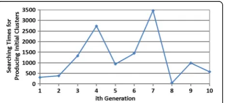
Tabu Search, the core of our algorithm, can solve the overlap problem of the initial cluster to improve its qual-ity. Ten Sequential Psim Matrix are generated, and the running time is shown in Fig. 2. After that, the corre-sponding initial clusters are generated in accordance with the method described in Section 3.3.2 and refined with the method in Section 3.3.3 to produce ten sets of refined
clusters. The searching times for producing the initial clusters are shown in Fig. 3. The overlap, recall, precision, and running time of the initial and refined clusters are cal-culated, respectively, as shown in Figs. 4, 5, 6 and 7.
It can be seen that 35–45% of the elements, which
were overlapping in the initial cluster, are eliminated by Tabu Search. The recall and precision of the initial clus-ter were approximately 39 and 34%, respectively. Afclus-ter Tabu Search, the recall reduced to approximately 33%, but the precision increased to approximately 39%. This is owing to the elimination of certain correct classified elements, while deleting the overlapping elements in the cluster, leading to a reduction in the recall. However, the number of error classified elements deleted by Tabu Search is more. Therefore, the proportion of correct classified elements in the cluster increases. The search-ing times for producsearch-ing the initial clusters is the random number from 1 to 5000, because the maximal searching timesCmaxis M= 5000. But in most cases, the expected
initial clusters can be found within 1500 times, and the corresponding running time is less than 9 s. The upper bound of running time for refining cluster is total time to construct all the permutations of cluster. In our ex-periment, the operation time is less than 0.5 s due to the limited number of clusters (only three clusters).
The experimental results are averaged and presented in Table 1; they illustrate the role of Tabu Search in the refinement of the initial cluster. After Tabu search, the precision increased from 33.9 to 38.4%, although the re-call reduced to 33.4%, satisfying the equilibrium distribu-tion of the precision and recall. In addidistribu-tion, several overlapping elements (approximately 40%) in the initial cluster are completely deleted with Tabu Search. The
Fig. 6Precision of the initial cluster and that of the refined cluster after running Tabu Search ten times
Fig. 7Running time of the initial cluster and that of the refined cluster after running Tabu Search ten times
Table 1Average performances of the initial and refined clusters with Tabu Search
Initial cluster Refined cluster
Overlap (%) 40.7 0
Recall (%) 39 33.4
Precision (%) 33.9 38.4
Running time (s) 7.36 0.49
average running time for producing the initial clusters is 7.36 s, and the one in refinement is 0.49 s. It can be seen that the time load from cluster optimization is accept-able. Therefore, it can improve the quality of the cluster to a certain extent.
4.4 Stability analysis
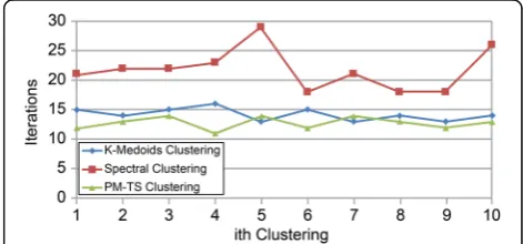
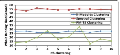
First, the method for determining the number of clus-ters, in Section 3.3.2, is applied to the test data. The re-sult is three, which corresponds to the existing data. Then, this dataset is clustered ten times with the PM-TS clustering algorithm, K-Medoids clustering algorithm [29], and the spectral clustering algorithm [26]. The cor-responding results are depicted in Figs. 8, 9, 10 and 11.
It can be seen that the iterations for the PM-TS clus-tering algorithm are lesser than those of the K-Medoids and spectral clustering algorithms, indicating that our proposed method can obtain a more precise initial clus-ter and converges fasclus-ter. In addition, the whole running speed of PM-TS clustering algorithm is faster than the one of K-Medoids and spectral clustering algorithms. In most cases, the clustering accuracy (Macro-F1 and Micro-F1) and stability (variations in Macro-F1 and Micro-F1) are both of the order, PM-TS clustering algo-rithm > spectral clustering algoalgo-rithm > K-Medoids clus-tering algorithm. The above results demonstrate the advantages of the PM-TS clustering algorithm in terms of the speed, accuracy, and stability. In some cases, the clustering accuracies of the K-Medoids and spectral clustering algorithms are less than 50%, indicating a
clustering failure. However, the PM-TS clustering algo-rithm did not have similar issues, exhibiting its validity.
4.5 Whole-performance analysis
The experimental results are averaged and presented in Table 2; they illustrate the better performance of the PM-TS clustering algorithm compared to the K-Medoids and spectral clustering algorithms. On the one hand, its iterations are lesser and the convergence is fast as well as the whole running speed. On the other hand, it has no failure cases and Macro-F1/Micro-F1 increase more than 13 and 10%, respectively. To sum up the above ana-lysis, the failure in the distance calculation, the ineffi-cient index tree, and the cluster overlap, derived from the characteristics of the high-dimensional data, can be corrected using the PM-TS clustering algorithm.
5 Conclusions
Audio signal clustering is critical in media computing. The key to improving its performance is the solving of the problems that exist in high-dimensional data cluster-ing, such as failures in the distance calculation, ineffi-cient index trees, cluster overlaps, etc. To address these problems, a clustering algorithm integrated with the se-quential Psim matrix, differential truncation, and Tabu Search is proposed. Compared to the other clustering al-gorithms, its characteristics are as follows: In high-dimensional space, the sequential Psim matrix is used to calculate the distance and organize data. Differential truncation and Tabu Search are used to obtain the initial cluster with a high accuracy. Experimental results indi-cate that the performance of this algorithm is better than
Fig. 9Whole running time of the three algorithms, run ten times Fig. 11Micro-F1 of the three algorithms, run ten times
Fig. 10Macro-F1 of the three algorithms, run ten times
Table 2Average performances of the three algorithms
K-Medoids clustering
Spectral clustering
PM-TS clustering
Iterations 14.2 21.8 12.8
Whole running time (s)
27.16 54.58 19.48
Macro-F1 (%) 50.71 46.94 59.81
that of the K-Medoids and spectral clustering algo-rithms. Several heuristic methods used in this algorithm have a potential for improvement. Thus, our future work includes the determination of more effective initial pa-rameters, evaluation functions, and convergence criteria, for improving the accuracy of the results.
Acknowledgements
We would like to thank Editage (www.editage.com) for English language editing and publication support.
Funding
This work is partly supported by the National Nature Science Foundation of China (No. 61502475) and the Importation and Development of High-Caliber Talents Project of the Beijing Municipal Institutions (No. CIT &
TCD201504039).
Availability of data and materials
The dataset supporting the conclusions of this article is available in the UCI database, http://archive.ics.uci.edu/ml/datasets/Waveform+Database +Generator+%28Version+2%29.
Authors’contributions
WL has conducted the research, analyzed the data, and authored the paper. GW has performed the overall design, providing new methods or models, and has written/revised the paper. All authors read and approved the final manuscript.
Ethics approval and consent to participate
Not applicable.
Consent for publication
Not applicable.
Competing interests
The authors declare that they have no competing interests.
Publisher’s Note
Springer Nature remains neutral with regard to jurisdictional claims in published maps and institutional affiliations.
Author details
1
College of Information Technology, Beijing Union University, No. 97 Beisihuan East Road, Beijing, China.2Institute of Biophysics, Chinese Academy of Sciences, No. 15 Datun Road, Beijing, China.
Received: 6 April 2017 Accepted: 23 November 2017
References
1. Ericson, K, & Pallickara, S. (2013). On the performance of high dimensional data clustering and classification algorithms.Futur. Gener. Comput. Syst., 29(4), 1024–1034.
2. Ravale, U, Marathe, N, Padiya, P. (2013). Attribute reduction based hybrid anomaly intrusion detection using K-means and SVM classifier.Int. J. Comput. Appl.,82(15), 32–35.
3. Gan, GJ, & Ng, MK. (2015). Subspace clustering using affinity propagation. Pattern Recogn.,48(4), 1455–1464.
4. Govaert, G, & Nadif, M (2014).Co-clustering: models, algorithms and applications. London: Wiley-ISTE.
5. Kriegel, HP, Kröger, P, Zimek, A. (2009). Clustering high-dimensional data: a survey on subspace clustering, pattern-based clustering, and correlation clustering.ACM Trans. Knowl. Discov. Data,3(1), 1–58.
6. Rashedi, E, & Mirzaei, A. (2013). A hierarchical clusterer ensemble method based on boosting theory.Knowl.-Based Syst.,45, 83–93.
7. Luo, R, & Yi, Q (2011). A novel parallel clustering algorithm based on artificial immune network using nVidia CUDA framework. InProceedings of the 14thinternational conference on human-computer interaction, (pp. 598–
607). Berlin: Springer-Verlag Press.
8. Sun, ZY, Mak, LO, Mao, KZ, Tang, WY, Liu, Y, Xian, KT, Wang, ZM, Sui, Y (2014). A knowledge-driven ART clustering algorithm. InProceedings of the IEEE International Conference on Software Engineering and Service Science 2014, (pp. 645–648). Birmingham: IEEE Comput Soc.
9. Keogh, E, & Mueen, A (2010). Curse of dimensionality. InEncyclopedia of machine learning, (pp. 257–258). Berlin: Springer-Verlag.
10. Yi, LH (2011).Research on clustering algorithm for high dimensional data. Qinhuangdao: Yanshan University.
11. Shahvari, O, & Logendran, R. (2017). An enhanced Tabu search algorithm to minimize a bi-criteria objective in batching and scheduling problems on unrelated-parallel machines with desired lower bounds on batch sizes. Comput. Oper. Res.,77, 154–176.
12. Tan, PN, Steinbach, M, Kumar, V (2005).Introduction to data mining. Boston: Addison-Wesley Publishing Company.
13. Yang, FZ, & Zhu, YY. (2004). An efficient method for similarity search on quantitative transaction data.J. Comput. Res. Dev.,41(2), 361–368. 14. Huang, SD, & Chen, QM. (2009). On clustering algorithm of high
dimensional data based on similarity measurement.Comput. Appl. Softw., 26(9), 102–105.
15. Shao, CS, Lou, W, Yan, LM. (2011). Optimization of algorithm of similarity measurement in high-dimensional data.Comput. Technol. Dev.,21(2), 1–4. 16. Wang, XY, Zhang, HY, Shen, LZ, Chi, WL. (2013). Research on high
dimensional clustering algorithm based on similarity measurement.Comput. Technol. Dev.,23(5), 30–33.
17. Jia, XY. (2005). A high dimensional data clustering algorithm based on twice similarity.J. Comput. Appl.,25(B12), 176–177.
18. Tan, N, & Shi, YX (2009). Optimization research of multi-dimensional indexing structure of R*-tree. InProceedings of the international forum on information technology and applications, (pp. 612–615). Berlin: Springer-Verlag Press.
19. Chen, HB, & Wang, ZQ. (2005). CR*-tree: an improved R-tree using cost model.Lect. Notes Comput. Sc.,3801, 758–764.
20. Nielsen, F, Piro, P, Barlaud, M (2009). Bregman vantage point trees for efficient nearest neighbor queries. InProceedings of the IEEE International Conference on Multimedia and Expo 2009, (pp. 878–881). Birmingham: IEEE Comput Soc.
21. Kunze, M, & Weske, M. (2011). Metric trees for efficient similarity search in large process model repositories.Lect. Notes Bus. Info. Proc.,66, 535–546. 22. Navarro, G. (2002). Searching in metric spaces by spatial approximation.
VLDB J.,11(1), 28–46.
23. Chen, JB (2011).The research and application of key technologies in knowledge discovery of high-dimensional clustering. Beijing: Publishing House of Electronics Industry.
24. Glover, F, & Laguna, M (2013). Tabu search*. InHandbook of combinatorial optimization, (pp. 3261–3362). Berlin: Springer-Verlag.
25. Li, WF, Wang, GM, Ma, N, Liu, HZ. (2016). A nearest neighbor search algorithm of high-dimensional data based on sequential Npsim matrix.High Technol. Lett.,22(3), 241–247.
26. Tremblay, N, Puy, G, Gribonval, R, Vandergheynst, P (2016). Compressive spectral clustering. InProceedings of the 33rdinternational conference on
machine learning, (pp. 1002–1011). Birmingham: IEEE Comput Soc. 27. Jin, X, & Han, JW (2010).K-Medoids clustering,Encyclopedia of machine
learning(pp. 564–565). New York: Springer Publishing. 28. Booth, TE. (2006). Power iteration method for the several largest
eigenvalues and eigenfunctions.Nucl. Sci. Eng.,154(1), 48–62. 29. Ng, RT, & Han, JW (1994). Efficient and effective clustering methods for
spatial data mining. InProceedings of the VLDB 1994, (pp. 144–155). Birmingham: IEEE Comput Soc.
30. Breiman, L, Friedman, J, Stone, CJ, Olshen, RA (1984).Waveform recognition problem,Classification and regression trees(pp. 64–66). Belmont: Wadsworth International Group.
31. Chen, LF, Ye, YF, Jiang, QS (2008). A new centroid-based classifier for text categorization. InProceeding of the IEEE 22ndInternational Conference on