R E S E A R C H
Open Access
Audio segmentation-by-classification
approach based on factor analysis in broadcast
news domain
Diego Castán
*, Alfonso Ortega, Antonio Miguel and Eduardo Lleida
Abstract
This paper studies a novel audio segmentation-by-classification approach based on factor analysis. The proposed technique compensates the within-class variability by using class-dependent factor loading matrices and obtains the scores by computing the log-likelihood ratio for the class model to a non-class model over fixed-length windows. Afterwards, these scores are smoothed to yield longer contiguous segments of the same class by means of different back-end systems. Unlike previous solutions, our proposal does not make use of specific acoustic features and does not need a hierarchical structure. The proposed method is applied to segment and classify audios coming from TV shows into five different acoustic classes: speech, music, speech with music, speech with noise, and others. The technique is compared to a hierarchical system with specific acoustic features achieving a significant error reduction.
Keywords: Audio segmentation; Factor analysis; Within-class variability compensation; Broadcast news; Albayzin 2010 evaluation
Introduction
Due to the increase in audiovisual content, it becomes necessary to use automatic tools for different tasks such as analysis, indexation, search, and information retrieval. Given an audio document, the first step is audio segmen-tation to obtain the delineation of a continuous audio stream into acoustically homogeneous regions. Secondly, each homogeneous region can be classified into prede-fined classes to provide labels that can be used as context for searching metadata or as identifiers for speaker adap-tation techniques in speech recognition systems.
Segmentation of broadcast news (BN) recordings into audio events (like speech, music, speech with music) is very challenging because such documents contain differ-ent kinds of sequences with a very heterogeneous style. Several international evaluation campaigns, like the TREC NIST evaluations for Spoken Document Retrieval (SDR) [1], the ESTER evaluations campaign for Rich Transcrip-tion (RT) in French [2], and the COST278 evaluaTranscrip-tion for segmentation and speaker clustering in multi-lingual
*Correspondence: [email protected]
Departamento Ingeniería Electrónica y Comunicaciones, Universidad de Zaragoza, María de Luna, 1, Zaragoza 50018, Spain
domain [3], have already been proposed to face this task in the past. Some examples of the audio sequences in BN (not pretending to be general definitions) in different conditions are as follows:
• News anchor speech : Traditional news anchor usually reading text in clean (or low-noise) conditions. • Interviews: Conversations between two people with
spontaneous speech or by following a script.
• Debates: Conversations between two or more people. They may contain overlapped speech in some parts. • Reporter in the field : The audio comes from a wide
range of noises generally overlapped with speech. • Advertising: Speech with music in background and a
variety of acoustic noise effects (slams, explosions, cars, screams, etc.).
• Jingles: Jingles are commonly used as a short tune to introduce different topics during the news.
• Broadcasting of sports events: Speech with a strong background noise and diegetic music and sounds. • Telephone connections: Used when the reporters do
not have camera and microphone.
The studies that can be found in the literature focus on either the feature extraction method or the segmenta-tion/classification strategies. A good review of the features
and the classification methods used in several solutions can be found in [4].
The proper selection of a set of acoustic features may help to describe the behavior of the acoustic classes (speech, music, environmental sounds, etc.) both in the time and frequency domains. Mel-frequency cepstrum coefficients (MFCC) or perceptual linear prediction (PLP) have been widely used throughout history in the context of audio and speech technologies [5-9] and more recently in [10]. More precisely, these features with other extended sets of features have been proposed for segmenting and classifying BN audio into broad classes. Among others, two pitch-density-based features are proposed in [11], short-time energy (STE) is used in [12-14], and harmonic features are used in [15-17]. The previously mentioned features are short-term characteristics because they are extracted within short periods of time (between 10 and 30 ms), usually known in the literature as frame-based features. These features are commonly used in speech-related tasks where the signal can be considered stationary over that short period. The frame-based features can be used directly in the classifier. However, some classes are better described by the statistics computed over consec-utive frames (from 0.5 to 5 s long). These characteristics are referred in the literature as segment-based features [18,19]. For example, in [20], a content-based speech dis-crimination algorithm is designed to exploit the long-term information inherent in the modulation spectrum. In [21], the authors propose two segment-based features: the vari-ance of the spectrum flux (VSF) and the varivari-ance of the zero crossing rate (VZCR).
Audio segmentation/classification systems can be divided into two different groups depending on how the segmentation is performed. The first group detects the boundaries in a first step and then classifies each delimited segment in a second step. We refer to them as segmentation-and-classification approaches. For exam-ple, in [22], an approach using a temporally weighted fuzzy C-means algorithm was proposed. The Bayesian information criterion (BIC) is widely employed in many studies as [23] to generate a break-point for every speaker change and environment/channel condition change in the BN domain. Also, [24] and [25] utilize BIC to identify mixed-language speech and speaker change, respectively. However, BIC has several shortcomings to be consid-ered. It can only set one break-point for each analysis window, so a small window involves more precision but the Gaussian estimation may be inaccurate due to the scarcity of data. In [26], the authors propose a minimum description length (MDL) approach that allows multiple break-points for any generic data. The second group is known as segmentation-by-classification and consists of classifying consecutive fixed-length audio segments. The segmentation is produced directly by the classifier as a
sequence of decisions. This sequence is usually smoothed to improve the segmentation performance. An example of this procedure can be found in [27] where the author combines different features with a Gaussian mixture model (GMM) and a maximum entropy classifier. The final decisions were smoothed with a hidden Markov model (HMM) to avoid sudden changes. In [28], an audio stream is segmented by classifying each window into five broad classes. The solution is a combination of different support vector machines (SVM) and evaluates the classi-fication over some new proposed features. Three different smoothing rules were applied to avoid sudden changes in the decisions. Aronowitz suggests a framework in which the classification and the smoothing are unified [29]. The author models the audio segments as supervectors, and each class (speech, silence, music) is modeled by a distri-bution over the supervector space. The supervectors are classified with SVM or GMM.
Segment-based features are not suitable for training sta-tistical models [21], and it is difficult to determinea priori the appropriate statistics for each class. However, they provide great discriminative power for audio classification if the segment is well-delimited using any segmentation-and-classification system [14]. On the other hand, frame-based features allow statistical models to make decisions over short-duration windows in segmentation-by-classification strategies [30], but they are usually less discriminative for audio classification since they were mainly designed for speech-related tasks such as auto-matic speech recognition (ASR) [21]. The most common solution to avoid the shortcomings and enjoy the bene-fits of each strategy is to create hierarchical systems with multiple steps where each level is designed with class-specific features and segmentation systems as in [31] and [32]. Nevertheless, these systems become very specific for the intended task and are quite difficult to adapt for other databases.
applied in speaker ID (recognition/verification) [34-38] and language recognition [39] with significant improve-ments with respect to GMM or SVM. However, the system proposed in this article has several differences from those systems. In contrast to a segmentation task, the speaker ID or language recognition has well-delimited segments (usually in separate files) and, therefore, FA is applied over the whole file. Unlike in the speaker ID, speaker diariza-tion, or language recognition tasks, we can find here the same speaker in two different acoustic classes, for exam-ple, the situation where an anchor is in the studio with clean conditions (SP) and outside of the studio with noise in the background (SN). Due to all these factors, we pro-pose an extension of a FA segmentation system propro-posed in [40] and [41] with a new and more discriminative scor-ing usscor-ing class/non-class parameters and with a set of back-end systems that perform a better segmentation than the traditional FA systems for language recognition or speaker ID.
The remainder of the paper is organized as follows: the database and metric of the Albayzin 2010 evalua-tion is presented in the ‘Albayzin audio segmentaevalua-tion evaluations and database description’ section. The ‘Novel factor analysis audio segmentation system’ section shows the theoretical approach based on FA and a set of back-end subsystems. The experiments are presented in the ‘Experimental results’ section. Finally, the summary and the conclusions are presented in the ‘Conclusions’ section.
Albayzin audio segmentation evaluations and database description
The Albayzin campaigns are internationally open evalua-tions organized by the RTTHaevery 2 years. A complete description of the Albayzin 2010 audio segmentation and classification evaluation can be found in [19] where the participant’s approaches and the results are presented. We describe the database and the metric used in the evaluation in the next subsections.
Database
The database consists of BN audio in Catalan recorded by the TALPbResearch Center. It includes approximately 87 h of annotated audio divided into 24 files. Five audio classes were defined for the evaluation. The classes are distributed as follows: clean speech, 37%; music, 5%; speech over music, 15%; speech over noise, 40%; others, 3%. The class ‘others’ is not evaluated in the final test. The database for the evaluation was split into two parts: for training (two thirds of the total amount of data divided into 16 files) and testing (the remaining one third divided into 8 files).
Each segment is labeled with one class previously described. Most of the segments are between 10 and 20 s long. However, there is an important amount of
long segments (longer than 60 s). More details about the database and the labeling process can be found in [19].
Metric
The metric that was proposed for the evaluation repre-sents the relative error averaged over all acoustic classes (ACs):
Error=averageidur(missi)+dur(fai)
dur(refi) , (1)
where dur(missi)is the total duration of all deletion errors (misses) for theith acoustic classes (AC), dur(fai) is the total duration of all insertion errors (false alarms) for the ith AC, and dur(refi)is the total duration of all theith AC instances according to the reference file. The incorrectly classified audio segment (a substitution) is computed both as a deletion error for one AC and an insertion error for another. A collar of 1 s is not scored around each refer-ence boundary to avoid the uncertainty about when an AC begins or ends.
Since the distribution of the classes in the database is not uniform, the errors from different classes are weighed dif-ferently (depending on the total duration of the class in the database). Therefore, the system has to detect correctly not only the best represented classes (‘speech’ and ‘speech over noise,’ 77% of total duration) but also the minor classes (like ‘music,’ 5%). This metric is different from the conventional NIST metric [42] for speaker diarization, where the score is defined as the ratio of the overall seg-mentation error time to the sum of the durations of the segments that are assigned to each class in the file. In this work, we will present the final results with both metrics.
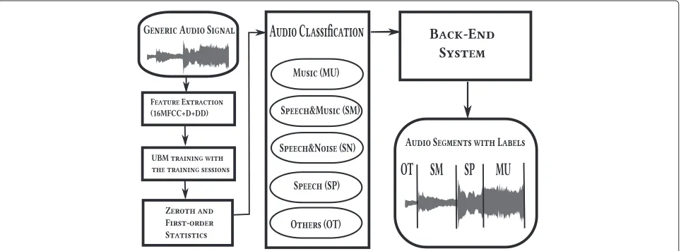
our task. Therefore, we introduce a novel approach with class/non-class parameters that compensate the within-class variability more accurately. Figure 1 illustrates the proposed framework where each block is described in the next subsections.
Acoustic feature extraction
In this work, we extract 16 MFCCs (including the zeroth-order cepstrum) computed in 25-ms frames with a 10-ms frame step and their first and second derivatives. The audio features are packed in windows of 3 s long with 0.1- or 0.5-s window steps depending on the desired computational load and resolution.
Statistics computation
The fixed-length windows are mapped to sufficient statis-tics by using a universal background model (UBM) [43] which is a class-independent GMM with C Gaussians estimated with the expectation-maximization (EM) algo-rithm [44] on the training data set. The UBM parameters are the mean vectors, μk, and the diagonal covariances matrices,k, wherekis the Gaussian component index. LetPksi = P(k|φsi)represent the posterior probability of thekth UBM component, given the feature vectorφsiand assuming frame independence [45]. For a windows, with feature vectors indexed i = 1, 2,. . .,Ns, we define the zeroth- and first-order statistics, respectively, as
nsk= Ns
i=1
Pksi, (2)
fsk= Ns
i=1
Pksi−k1/2φsi−μk, (3)
where these statistics are normalized to the UBM.
Theoretical background
Data from a particular class are modeled by a GMM defined by a set of mean vectorsm1,m2,. . .,mC, weights w1,w2,. . .,wC, and covariance matrices 1,2,. . .,C, whereCis the number of Gaussians. We can concatenate all GMM mean vectors to one mean supervector m of dimensionCF×1 whereFis the feature vector length:
m=
mT1,mT2,. . .,mTC
T
. (4)
The factor analysis model is the adaptation of the UBM model where the supervector of means is not fixed and it can vary from segment to segment due to several sources that increase the within-class variability [36]. We assume that these GMMs have segment- and class-dependent means but fixed weights and covariances chosen to be equal to the UBM weights and covariances. Specifically, we use a factor analysis model for the mean vector of the kth component of the GMM for segments:
mks =tkc(s)+Ukxs, (5)
wherec(s)denotes the class of segments. The class loca-tion vector tkc(s) is obtained by using a single iteration of relevance MAP adaptation from the UBM [43]. This adaptation is expressed, in terms of statistics, as
tck(s)=
sfsk
r+snsk
, (6)
where ris the relevance factor. Uk is the factor loading matrix andxsis a vector ofL segment-dependent-within-class-variability factors assumed to follow a normal distri-bution(N(0,IL)).
We stack the component-dependent vectors into super-vectors ms and tc(s) and the component-dependent Uk
matrices into a single tall matrixU, so Equation 5 can be expressed as
ms=tc(s)+Uxs, (7)
whereU is known as the within-class variability matrix that we use to compensate that variability. The columns of the U matrix are the basis spanning the subspace of the within-class variability, and the within-class variabil-ity factors are the coordinates defining the position of the supervector in the subspace. The within-class variability factor dimension (L) is smaller thanCF, soUhas low rank (CF×Ldimensions). Depending on the application, the value ofLis between 50 and 200 andCFcan be 98,304 if we have 2,048 Gaussians and 48-dim feature vector (with the MFCC-UBM).
Estimation of the within-class variability matrices
U can be estimated using the EM algorithm, where the xfactors of each window are treated as hidden variables. In the E step, the expected value ofx(denoted byxˆ) are estimated for each window, using the current parameters as
ˆ xs=
I+
k
nskUTkUk −1
UTfs. (8)
In the M step, we obtainU that maximize an auxiliary function involving the old and new parameters as
Uk=
c
s
fsk−tck(s)nsk
ˆ xTs
A−k1, (9)
where
Ak=
s
ˆ xsxˆTs
T
nsk. (10)
This paper does not aim to deepen into the training pro-cess ofU; more details and an exhaustive description can be found in [36].
Class model vs alternative model U matrices
The approach proposed in this paper has several differ-ences with language recognition in the way within-class variability is compensated. Most of the approaches based on FA for language recognition are implemented with a singleUmatrix because the segments are well-delimited (typically in separated files) and the nature of the within-class variability is similar for all the languages as it can be seen in [36,46-48]. In [49], a segmentation system was pro-posed with five class location vectors (one vector per class) and a single compensation matrix U for all the classes. The paper compared the FA system with the winner of the Albayzin 2010 evaluation, and the conclusion was that the FA system is better as a classification system with oracle segments. On the other hand, the compensation matrix
had a bad behavior in a segmentation-by-classification system for the music class due to the different nature of the rest of the classes. In [32], a hierarchical system was proposed with different features and different techniques in each level depending on the class. First, the system decides among MU, SM, or the rest of the classes by using HMM/GMM and a smoothed combination of MFCC and Chroma as feature vectors. Next, the system classifies SP and SN by using FA and MFCC as acoustic features to improve the performance of the speech classes because the confusion between these two classes is very high. The error rate achieved was lower than the one obtained by the best system presented in the Albayzin 2010 evaluation showing a clear advantage when the classes are homo-geneous (like SN and SP), sinceU models the variability across speakers and phonemes. The background noise is, then, the discriminative information for the classification and segmentation. Nevertheless, hierarchical systems can be very specific for an intended task and are difficult to adapt to other databases with new classes.
Therefore, we propose here a non-hierarchical segmentation-by-classification system with ten class-specific vectors (one class vector and one non-class vector for each class) and five matrices modeling the within-class variability of each pair class/non-class. Let
T =
tMU,tMU,tOT,tOT,
tSM,tSM,tSN,tSN,tSP,tSP
(11)
and
= UMU−MU,UOT−OT,
USM−SM,USN−SN,USP−SP
, (12)
whereTrepresents the locations of classes (tC) and non-classes (tC) in the GMM space and the within-class variability matrices. This approach will be compared to the classic formulation with a singleU matrix in ‘Experi-mental results’ section for the classification over the oracle segments and the final segmentation system.
Scoring
We study here the two scoring approaches most commonly used: the integration over thexfactors distri-butions and the linear scoring, both of which are summa-rized in [50].
Score 2: The linear scoring, which is faster than the previous one, is an approximation that makes use of the first-order Taylor expansion [50].
In [50,51] and [36], the score employed to detect the speaker is the log-likelihood ratio test (LLRT)
LLRTclass=log
P(χ/class)
P(χ/UBM), (13)
where the numerator is the likelihood for the class model and the denominator the likelihood for the UBM. Note that the UBM is used as a general model to describe the alternative hypothesis which is appropriated for speaker identification where the hypothesized speaker is not in the UBM. However, our problem has a small number of classes, and therefore, each class is highly represented by the UBM and may corrupt the test statistics.
We propose here a compensated log-likelihood ratio test (CLLRT) scoring:
CLLRTclass=log
P(χ/class)
P(χ/class), (14)
where the alternative hypothesis is the likelihood for the non-class model which is compensated also with the with-in class variability matrix. The CLLRT is expected to be more discriminative than the LLRT for a segmentation task because the hypothesized class is not present in the denominator and, also, because the non-class model is compensated in the same way as the class model.
Back-end systems
We propose here three different back-end systems to com-bine, smooth, and improve the classification performance of the FA:
1. Maximum a posteriori (MAP) : This well-known method has been widely used in the literature [40,41]. To increase the detection performance, we optimize the prior probabilities in a Viterbi algorithm over the training files. Later, these priors are
employed in the Viterbi over the test files. 2. Derivative HMM/GBE : There is an apparent
correlation among the likelihood ratios of different classes. For example, if a segment is a jingle, the likelihood ratio for the MU class (music) should be the biggest, but it is very likely that the second one is the SM (speech with music). Also, SN (speech and
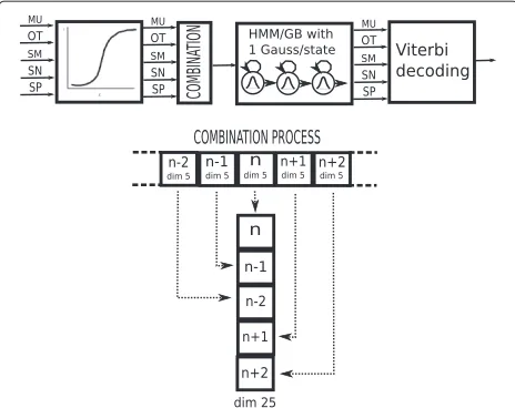
noise) and SM (speech with music) are more correlated between them than to the SP class (speech) because both classes have background audio. The classification and, therefore, the segmentation can be improved by combining the outputs of each class-dependent subsystem [52]. Figure 2 shows the combination and smoothing back-end system proposed here. On a first step, a calibration of scores is made by a multi-class logistic regression [53] estimated using the training partition of the database. In order to benefit from the use of the dynamic behavior of the scores, we compute the first- and second-order time derivatives of the scores. To smooth the decisions after the calibration and the dynamic description, one Gaussian/HMM back-end is used for each class. A left-to-right topology was selected with a full-covariance Gaussian per state estimated with the scores from the training files. The mean vectors and the covariance matrices are estimated with the samples of the scores based on the class labels with the ML criterion. The number of states for the HMM depends on the desired level of smoothing. The Viterbi algorithm was chosen to determine the maximum likelihood transitions between the classes.
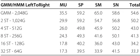
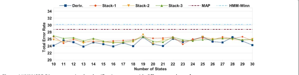
3. Stacking HMM/GBE : This back-end system can be considered as a modification of the previous back-end system. The main idea is to provide contextual information through longer term temporal scoring. Instead of the derivation of the scores, this back-end system proposes a stacking of past and future scores with the present score to model the dynamic behavior in a different way. Figure 3 shows this combination process where several score frames from the past and several score frames from the future are stacked with the present frame. The experiments are carried out with one, two, and three frames from the past and future and different numbers of states.
In an HMM segmentation system, it is usual to opti-mize the transition penalties on a development set since this can have a significant impact on performance. How-ever, we do not optimize any transition penalty because our goal was to create a general approach to segment audio that could be used in other databases with different distributions or with other classes.
Figure 3Back-end system 3 - stacking HMM/GBE block diagram.
Experimental results
The errors can be produced in two ways: first, a clas-sification error due to a bad labeled frame, and a seg-mentation error due to a temporal mismatch between the reference boundaries and the hypothesis boundaries. This section shows the experiments for the evaluation data described in the ‘Albayzin audio segmentation evaluations and database description’ section divided into two sets. In the first set, the boundaries between segments are given by the ground truth and the system decides the class of each segment with no segmentation error to evaluate the classification accuracy of the classical FA system versus GMMs.
The second set of experiments shows the segmenta-tion and the classificasegmenta-tion error when the boundaries are not given. A final segmentation-by-classification system based on FA with a class/non-class parameters is pro-posed. The three back-end systems previously described are tested over this system. The back-end systems show that a combination and smoothing of the scores improve the previous results. Also, the systems are compared to the winner system of the 2010 Albayzin evaluation that has a hierarchical structure with specific features for each class.
Classification experiments with oracle segmentation The classification is made over the segments extracted with the ground truth boundaries to evaluate the classifi-cation accuracy over the whole segment. Since the system decides the class that the whole segment belongs to, the smoothing is not needed.
We propose GMM systems as a baseline for classifica-tion experiments using the acoustic features described in the ‘Acoustic feature extraction’ section. Table 1 shows the results for these systems. We have evaluated different
Table 1 Baseline for classification experiments
GMM MU SP SM SN Total
64G 10.68 45.74 36.68 45.44 34.63
128G 9.81 41.79 32.02 40.75 31.09
256G 10.4 37.6 31.8 37.6 29.3
512G 9.5 35.9 29.3 35.9 27.7
1,024G 9.3 34.9 27.0 34.3 26.4
2,048G 9.6 33.3 28.0 34.0 26.2
Classification error per class and total error for GMM systems with different numbers of Gaussians over the test files with perfect segmentation. The italicized number represents the best performance of the GMM system.
numbers of Gaussians (from 64 to 2,048). The classifi-cation is based on the highest accumulated likelihood over the whole segment. As it can be seen in Table 1, increasing the number of Gaussians improves the final result. The highest number of Gaussians evaluated was 2,048 because the error for MU and SM classes began to increase although the total result improved slightly compared to the 1024G model.
In the experiments with FA for classification with oracle segmentation, we assess different configurations for the number ofxfactors and the scoring methods described previously. The UBM employed to compute the statis-tics has a fixed number of 2,048 Gaussians to be able to compare the results of the FA systems with the best GMM baseline configuration. Because the boundaries are known, the statistics are calculated over the whole seg-ment without merging underlying partitions. We compute the result using linear scoring and the integration trough the x factors distributions scoring (called as IoChD in this section). The linear scoring needs a final calibration because the scoring is scaled by the module of the tar-get model. A Gaussian back-end (GBE) ([54,55]) provides benefits in two ways: calibration and score combination. The calibration for the IoChD scoring does not provide substantial benefits because the score is based on a like-lihood ratio over a MAP adaptation using the same UBM and the marginal improvement comes from the combi-nation of scores. The experiments are carried out with a singleU matrix to compensate all the within-class vari-ability and different numbers ofx factors (50, 100, 150, 200, 250, and 300) providing the error for each class. Note that the increment of x factors involves an exponential increment of the computational cost.
Table 2 FA systems for classification experiments
One U for all classes
Linear GBE IoChnf
Number of chnf MU SP SM SN Total MU SP SM SN Total
50 21.6 16.9 23.6 23.4 21.4 10.2 15.9 24.2 21.4 17.9
100 21.8 17.4 21.0 22.9 20.8 9.1 16.0 20.2 20.0 16.3
150 20.8 17.7 20.5 23.5 20.6 9.4 15.5 18.0 18.9 15.4
200 20.7 17.8 20.5 22.4 20.4 9.0 15.7 17.3 19.1 15.3
250 20.0 19.2 20.2 23.1 20.6 8.5 16.7 16.0 19.4 15.1
300 21.3 19.5 20.5 21.7 20.8 9.8 15.0 18.9 18.9 15.6
Classification error per class and total error for linear and IoChD scoring with perfect segmentation and a single U for all the classes. The italicized numbers represent the best performance of the FA system for a given configuration.
the total result (18.3% relative error reduction with linear scoring and 50xfactors) and also compared to the best FA configuration (43.1% relative error reduction with IoChD scoring and 150xfactors). Note that the music has been better classified with GMMs than with linear GBE. How-ever, the rest of the classes presents a high classification error with GMMs (as we knew from the results presented in the Albayzin evaluation).
An important fact about the distribution of the errors is shown in Table 3. The table shows the percentages of the segments that have been correctly classified for GMM with 2,048 Gaussians, FA with linear GBE scoring and FA with IoChD scoring both with 100 channel factors. The table is divided into two columns: the first column shows the percentage of the correctly classified segments between 0 and 3 s long. It clearly shows that, while the classification is better with FA systems as we have shown in Table 2, segments shorter than 3 s are better classified with GMMs. The second column shows the percentage of the segments longer than 3 s. It can be seen that the best classification system is based on FA with IoChD scoring. As a conclusion, the FA is a better classifier if the segments are longer than 3 s which is a common fact because most of the segments are between 10 and 20 s long and a collar of 1 s is not scored around each reference boundary.
Segmentation-by-classification experiments
In this subsection, no oracle segment boundaries are con-sidered, so the audio stream is segmented by classifying each window into one of the five classes.
Table 3 Percentage of correctly classified segments shorter than 3 s and longer than 3 s
Segment<3 s Segment≥3 s
GMM - 2,048G 25.4 56.9
Linear GBE - 100 chnf 19.2 57.3
IoChnf - 100 chnf 23.4 60.8
The total number of segments is 7,754. The italicized numbers represent the best performance for segments shorter than 3 s and longer than 3 s.
Table 4 shows the baseline results for this segmentation task. To be able to compare the results with the best base-line classification system of Table 1, the basebase-line segmen-tation systems in Table 4 are based on GMM with 2,048 Gaussians. The first row in this table shows the results of a basic GMM - 2,048G system. The segments in this system are delimited by the transition of the frame-by-frame classification and no smoothing is applied. Note the degradation of the GMM - 2,048G (54.6% of total error) compared to the GMM - 2,048G with perfect segmenta-tion in Table 1 (26.2% of total error) where the decision of each class was based on the accumulated likelihood of the whole given segment. These results clearly show that a smoothing stage to avoid sudden changes in the deci-sion sequence is needed in a segmentation task. A widely used technique to smooth the transitions between classes is the left-to-right HMM topologies. Table 4 shows differ-ent left-to-right HMM configurations where the 2,048G are divided by the number of states to maintain the same number of Gaussians in every configuration. The best baseline system for the segmentation task (33.3% of total error) has 32 states with 64G per state (keeping a total of 2,048G). This result proves the dramatic improvement when a temporal smoothing is applied to segmentation-by-classification system.
Classification experiments in the last subsection indi-cate that the IoChD scoring is more accurate than the
Table 4 Baseline for segmentation experiments
GMM/HMM LeftToRight MU SP SM SN Total
GMM - 2,048G 35.5 59.2 65.0 58.6 54.6
2 ST - 1,024G 29.9 59.2 54.7 56.8 50.2
4 ST - 512G 26.0 49.8 45.9 50.2 43.0
8 ST - 256G 24.3 49.3 41.6 50.1 41.3
16 ST - 128G 17.8 40.2 36.0 43.0 34.2
32 ST - 64G 17.3 39.5 33.9 41.5 33.3
Table 5 Error per class and total error for FA segmentation-by-classification systems
IoChD scoring: step - 0.5 s, 100 chnf
MU SP SM SN Total
One single U 40.3 76.9 60.5 64.3 60.5
One U per class 33.3 45.6 36.2 47.4 40.6
The experiments are computed with one single U for all the classes and one U matrix for each class/non-class using IoChD scoring. No score combination or smoothing was carried out. The italicized numbers show the total error of each system.
linear scoring as we asserted in the ‘Scoring’ section. For the sake of clarity, results with the linear scoring are not presented in this subsection.
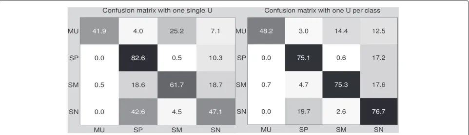
Unlike the oracle segmentation where thexfactors were computed for each segment, in this subsection thex fac-tors are computed for each window, so an increment in the number of x factors or a reduction of the window step increases the memory and the time needed to train the models dramatically. As a preliminary experiment, the FA segmentation-by-classification system computes the statistics every 0.5 s and 100xfactors. Because the win-dows (3 s long in our experiments) are smaller than the oracle segments, the useful information which describes the class of the window is scarcer. Therefore, a more dis-criminative scoring is needed and it is provided by the models with one U matrix for each class. Results with a single U matrix for all the classes and one U matrix for each class are presented in Table 5. There is a signifi-cant improvement in the classes with more data using one U matrix for each class because the CLLRT removes the information of the target class in the denominator as we pointed out in the ‘Scoring’ section. Figure 4 displays the confusion matrices for the experiments of Table 5. The percentages have been computed with the frames scored (affected by the collar) divided by all the frames of each class in the reference (dur(refi)). The table clearly shows
less confusion between classes using one U matrix for each class. Specially, there is a significant reduction in the confusion between SP and SN and a slight reduction in the confusion between MU and SM. The more frequent the class in the data, the more significant the error reduc-tion compared to a single U matrix for all the classes. Accordingly, the total error is reduced around 20%.
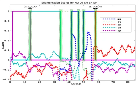
Once the benefits of the FA system with oneU matrix for each class with IoChD scoring are determined, the window-step can be reduced to increase the resolution (0.1-s window step) at the expense of increasing the com-putational cost. The number ofxfactors is not increased because the computation time and the memory grow exponentially. Figure 5 shows the scores for each class over a chunk of a test file. The ground truth is plotted in the same figure, and it is represented with a square wave of amplitude 1. The green bars represent the forgive-ness collar around each boundary. The color of each score class and the corresponding ground truth is the same. The figure clearly shows that the ratio of the winner class is bigger than zero and corresponds to the ground truth class for most of the frames. The results in Table 5 can be compared to the results in Table 6 showing a significant error reduction achieved by decreasing the window step because of the resolution increase.
To avoid sudden changes in the segmentation process, three back-end subsystems are evaluated here. The first back-end system is based on a MAP approach, and the two following systems are very similar but they model the temporal behavior in different ways: on a first step, the scores of both systems are conditioned using a multi-class logistic regression. The dynamic behavior of the scores is extracted with the first- and second-order time deriva-tives or by stacking the past and future frames of the scores (we know these systems as derivative HMM/GBE and stacking HMM/GBE, respectively). Finally, a left-to-right HMM/GBE with full covariance matrices is used to smooth the scores and improve the results with a scoring
Figure 5Scores and ground truth of each class over a chunk of a test file.
combination for both systems. The number of states in the HMM determines the minimum length of the segment.
We compare the error of the system proposed in this work with the winner system of the Albayzin 2010 evalu-ation [31] where 15 MFCCs, frame energy, and their cor-responding first and second derivatives are extracted. In addition, the spectral entropy and the Chroma coefficients are calculated. The mean and variance of these features are computed over 1-s intervals creating 122 dimension feature vectors. The segmentation approach chosen is HMM-based. The acoustic modeling is performed using five HMMs with three emitting states and 256 Gaussians per state. Each HMM corresponds to one acoustic class. A hierarchical organization of binary HMM detectors is used. First, audio is segmented into music/non-music
Table 6 Error per class and total error for FA segmentation-by-classification systems
IoChD scoring: step - 0.1 s, 100 chnf
MU SP SM SN Total
One U per class 27.9 37.9 32.4 40.9 34.8
The experiments are computed with one U matrix for each class/non-class using IoChD scoring. No score combination or smoothing was carried out. The italicized number shows the total error of the system.
portions. Second, the non-music portions are further seg-mented into speech-over-music/non-speech-over-music portions. Finally, the non-speech-over-music portions are segmented into speech/speech over noise.
Figure 6HMM/GBE-FA segmentation-by-classification system with different numbers of states.
Table 7 is divided into two parts: the first part shows the error for each class and the average error for the win-ner hierarchical-HMM system of the evaluation (HMM-Winn). The last column shows the NIST metric used in the NIST RT Diarization evaluations [42] to com-pare the systems with a well-known metric. To be able to compute the NIST error with the hierarchical-HMM system, we replicated the winner system according to [31] (HMM-Rep). The second part of the table shows the FA segmentation-by-classification system (FA-Segm) after the combination and the smoothing with the deriva-tive HMM/GBE back-end subsystem because this subsys-tem is slightly better than the other back-end subsyssubsys-tems. We choose the best configuration (Best FA-Segm) and the worst configuration (Worst FA-Segm). Note that the final number of states is not very critical because the difference between errors is less than 3%. The best result obtained was an error of 23.8% using 13 states, and the worst result was 26.6% with 25 states. The hierarchical-HMM systems perform better than the worst FA system for the MU and SM classes, but their behavior is worse for SN and SP. Also, there is not a substantial benefit classifying the MU with the best FA system compared to the hierarchical-HMM system. This is due to the use of specific features to detect the music like the Chroma features. The worst FA system achieves a relative error reduction of 11.3% with respect to the hierarchical-HMM system. Finally, the best FA config-uration improves the performance for all the classes and achieves a relative error reduction of 29.2% with respect to the hierarchical-HMM system.
Conclusions
This paper presents a novel system to segment and clas-sify audios coming from broadcast TV news into five broad classes. The proposed system is based on a fac-tor analysis (FA) approach to compensate the within-class variability with one factor loading matrix per class. Unlike other FA systems (like speaker ID and language recog-nition), the system proposed in this work does not have well-delimited segments, the same speaker can be found in different classes, and the nature of the classes can be very different (music, speech, or noise). The relevance of this approach can be summarized in two major aspects: it does not need specific features or hierarchical struc-ture and it performs a very accurate segmentation and classification for all the classes. Therefore, the system is general enough to be used for different tasks and scenar-ios. The classification experiments with oracle tation (‘Classification experiments with oracle segmen-tation’ section) show a clear improvement compared to the baseline GMM system. A class/non-class FA system is proposed for the segmentation-by-classification experi-ments in the ‘Segmentation-by-classification experiexperi-ments’ section. Different back-end systems have been evaluated in order to exploit the correlation among classes and avoid sudden changes in the decisions. This system is com-pared to a hierarchical solution with specific features for each level. The results show a significant improvement for all classes, metrics, and configurations achieving a 29.2% relative error reduction with respect to the hierarchical-HMM system for the best configuration.
Table 7 Results for the Albayzin evaluation winner system and factor analysis segmentation system over the test files
Error for each class
MU SP SM SN Total NIST
HMM-Winn [31] 19.2 39.5 25.0 37.2 30.2
-HMM-Rep 16.3 40.8 24.0 38.8 30.0 19.3
Worst FA-Segm 19.3 29.5 24.6 33.1 26.6 16.7
Best FA-Segm 18.8 23.7 23.6 29.1 23.8 14.7
Endnotes
aSpanish Thematic Network on Speech Technologies:
http://www.rthabla.es.
bThe Center for Language and Speech Technologies
and Applications (TALP) is a specific interdepartmental research center at the Technical University of Catalonia.
Abbreviations
AC, acoustic classes; BN, broadcast news; HMM, hidden Markov model; GMM, Gaussian mixture model; FA, factor analysis; UBM, universal background model.
Competing interests
The authors declare that they have no competing interests.
Acknowledgements
This work has been funded by the Spanish Government and the European Union (FEDER) under the project TIN2011-28169-C05-02.
Received: 7 March 2014 Accepted: 30 June 2014 Published: 28 August 2014
References
1. NIST, TREC NIST Evaluations. http://www.itl.nist.gov/iad/mig//tests/sdr/. Accessed 6 Aug 2014
2. S Galliano, E Geoffrois, D Mostefa, The ESTER phase II evaluation campaign for the rich transcription of French broadcast news, in
Interspeech,Lisbon, 4–8 Sept 2005, pp. 3–6
3. J Zibert, F Mihelic, J Martens, H Meinedo, J Neto, L Docio, C Garcia-Mateo, P David, E Al, The COST278 broadcast news segmentation and speaker clustering evaluation-overview, methodology, systems, results, in
Interspeech,Lisbon, 4–8 Sept 2005
4. Y Lavner, D Ruinskiy, A decision-tree-based algorithm for speech/music classification and segmentation. EURASIP J. Audio Speech Music Process.
2009, 1–15 (2009)
5. S Imai, Cepstral analysis synthesis on the mel frequency scale, inIEEE International Conference on Acoustics, Speech, and Signal Processing
Conference Proceedings,Boston, 14–16 Apr 1983, pp. 93–96
6. R Vergin, D O’Shaughnessy, V Gupta, Compensated mel frequency cepstrum coefficients, inIEEE International Conference on Acoustics,
Speech, and Signal Processing Conference Proceedings,vol. 1, Atlanta, 7–10
May 1996, pp. 323–326
7. R Vergin, Generalized mel frequency cepstral coefficients for
large-vocabulary speaker-independent continuous-speech recognition. IEEE Trans. Speech Audio Process.7(5), 525–532 (1999)
8. E Wong, S Sridharan, Comparison of linear prediction cepstrum coefficients and mel-frequency cepstrum coefficients for language identification, inInternational Symposium on Intelligent Multimedia, Video
and Speech Processing,Kowloon Shangri-La, Hong Kong, 2–4 May 2001,
pp. 95–98
9. M Hasan, M Jamil, M Rahman, Speaker identification using mel frequency cepstral coefficients, inInternational Conference on Computer and Electrical
Engineering,Dhaka, 28–30 Dec 2004
10. P Dhanalakshmi, S Palanivel, V Ramalingam, Classification of audio signals using AANN and GMM. Appl. Soft Comput.11(1), 716–723 (2011) 11. L Xie, Z-H Fu, W Feng, Y Luo, Pitch-density-based features and an SVM
binary tree approach for multi-class audio classification in broadcast news. Multimed. Syst.17(2), 101–112 (2011)
12. J Saunders, Real-time discrimination of broadcast speech/music, inIEEE International Conference on Acoustics, Speech, and Signal Processing
Conference Proceedings,Atlanta, 7–10 May 1996, pp. 993–996
13. D Li, I Sethi, N Dimitrova, T McGee, Classification of general audio data for content-based retrieval. Pattern Recogn. Lett.22, 533–544 (2001) 14. L Lu, H Zhang, H Jiang, Content analysis for audio classification and
segmentation. IEEE Trans. Speech Audio Process.10(7), 504–516 (2002) 15. TL Nwe, H Li, Broadcast news segmentation by audio type analysis, inIEEE
International Conference on Acoustics, Speech and Signal Processing,vol. 2,
Philadelphia, 18–23 Mar 2005, p. 1065
16. A Hauptmann, R Baron, M Chen, Informedia at TRECVID 2003: analyzing and searching broadcast news video, inProc. TRECVID,Gaithersburg, 17–18 Nov 2003
17. S Dharanipragada, M Franz, Story segmentation and topic detection in the broadcast news domain, inDARPA Broadcast News Workshop, Herndon, 28 Feb–3 Mar 1999, pp. 1–4
18. A Gallardo-Antolín, J Montero, Histogram equalization-based features for speech, music, and song discrimination. IEEE Signal Process. Lett.
17(7), 659–662 (2010)
19. T Butko, C Nadeu, Audio segmentation of broadcast news in the Albayzin-2010 evaluation: overview, results, and discussion. EURASIP J. Audio Speech Music Process.2011(1), 1 (2011)
20. M Markaki, Y Stylianou, Discrimination of speech from nonspeeech in broadcast news based on modulation frequency features. Speech Commun.53(5), 726–735 (2011)
21. R Huang, J Hansen, Advances in unsupervised audio classification and segmentation for the broadcast news and NGSW corpora. IEEE Trans. Audio Speech Lang. Process.14(3), 907–919 (2006)
22. N Nguyen, M Haque, C-h Kim, J Kim, Audio segmentation and
classification using a temporally weighted fuzzy C-means algorithm. Adv. Neural Netw.6676, 447–456 (2011)
23. SS Chen, PS Gopalakrishnan, Speaker, environment and channel change detection and clustering via the Bayesian information criterion, inProc.
DARPA Broadcast News Workshop,Lansdowne, 8–11 Feb 1998
24. C-h Wu, Y Chiu, Automatic segmentation and identification of mixed-language speech using delta-BIC and LSA-based GMMs. IEEE Trans. Audio Speech Lang. Process.14(1), 266–276 (2006)
25. M Kotti, E Benetos, C Kotropoulos, Computationally efficient and robust BIC-based speaker segmentation. IEEE Trans. Audio Speech Lang. Process.
16(5), 920–933 (2008)
26. C-h Wu, C-h Hsieh, Multiple change-point audio segmentation and classification using an MDL-based Gaussian model. IEEE Trans. Audio Speech Lang. Process.14(2), 647–657 (2006)
27. A Misra, Speech/nonspeech segmentation in web videos, inProc.
Interspeech,Portland, 9–13 Sept 2012
28. L Lu, H-J Zhang, SZ Li, Content-based audio classification and segmentation by using support vector machines. Multimed. Syst.
8(6), 482–492 (2003)
29. H Aronowitz, Segmental modeling for audio segmentation, inIEEE International Conference on Acoustics, Speech, and Signal Processing
Conference Proceedings,Honolulu, 15–20 Apr 2007, pp. 393–396
30. J Foote, A similarity measure for automatic audio classification, in American Association for Artificial Intelligence: Intelligence Integration and
Use of Text, Image, Video, and Audio Corpora(Stanford, March 1997)
31. A Gallardo, R San Segundo, UPM-UC3M system for music and speech segmentation, inII Iberian SLTech,Vigo, 10–12 Nov 2010, pp. 421–424 32. D Castan, C Vaquero, A Ortega, D Martínez, E Lleida, Hierarchical audio
segmentation with HMM and factor analysis in broadcast news domain,
inProc. Interspeech,Florence, 15 Aug 2011
33. T Butko, CN Camprubí, H Schulz, Albayzin-2010 audio segmentation evaluation: evaluation setup and results, inII Iberian SLTech,Vigo, 10–12 Nov 2010, pp. 305–308
34. P Kenny, G Boulianne, P Dumouchel, Eigenvoice modeling with sparse training data. IEEE Trans. Speech Audio Process.13(3), 345–354 (2005) 35. P Kenny, Joint factor analysis of speaker and session variability: theory and
algorithms, 1–17 (2006). http://www.crim.ca/perso/patrick.kenny. Accessed 6 Aug 2014
36. P Kenny, G Boulianne, P Ouellet, P Dumouchel, Joint factor analysis versus eigenchannels in speaker recognition. IEEE Trans. Audio Speech Lang.
15(4), 1435–1447 (2007)
37. C Vaquero, A Ortega, J Villalba, A Miguel, E Lleida, Confidence measures for speaker segmentation and their relation to speaker verification, inProc
Interspeech 2010,vol. 2010, Makuhari, 26–30 Sept 2010, pp. 2310–2313
38. C Vaquero, A Ortega, E Lleida, Intra-session variability compensation and a hypothesis generation and selection strategy for speaker segmentation,
inIEEE International Conference on Acoustics, Speech and Signal Processing,
Prague, 22–27 May 2011, pp. 3–6
39. N Brummer, A Strasheim, V Hubeika, P Matˇejka, L Burget, O Glembek, Discriminative acoustic language recognition via channel-compensated GMM statistics, inProc Interspeech,Brighton, 6–10 Sept 2009,
pp. 2187–2190
41. D Castan, A Ortega, J Villalba, E Lleida, Segmentation-by-classification system based on factor analysis, inIEEE International Conference on Acoustics, Speech, and Signal Processing Conference Proceedings, Vancouver, 26–31 May 2013
42. NIST,The 2009 (RT-09) Rich Transcription Meeting Recognition Evaluation Plan, (Melbourne, 28–29 May 2009
43. D Reynolds, TF Quatieri, RB Dunn, Speaker verification using adapted gaussian mixture models. Digit. Signal Process.10(1–3), 19–41 (2000) 44. CM Bishop,Pattern Recognition and Machine Learning, vol. 4. Computers
-Springer, Aug 17, 2006, p. 738
45. P Kenny, D Reynolds, F Castaldo, Diarization of telephone conversations using factor analysis. IEEE J. Selected Topics Signal Process.
4(6), 1059–1070 (2010)
46. H Li, B Ma, K Lee, Spoken language recognition: from fundamentals to practice. Proceedings of IEEE.101(5), 1136–1159 (2013)
47. F Castaldo, D Colibro, E Dalmasso, P Laface, C Vair, Compensation of nuisance factors for speaker and language recognition. IEEE Trans. Audio Speech Lang. Process.15(7), 1969–1978 (2007)
48. R Vogt, S Sridharan, Explicit modelling of session variability for speaker verification. Comput. Speech Lang.22(1), 17–38 (2008)
49. D Castan, A Ortega, E Lleida, Factor analysis segmentation and classification in broadcast news domain, inProc. III Iberian SLTech,Madrid, 21–23 Nov 2012
50. O Glembek, L Burget, N Dehak, N Brummer, P Kenny, Comparison of scoring methods used in speaker recognition with joint factor analysis, in IEEE International Conference on Acoustics, Speech and Signal Processing, Taipei, 19–24 Apr 2009, pp. 4057–4060
51. P Kenny, G Boulianne, P Ouellet, P Dumouchel, Factor analysis simplified,
inIEEE International Conference on Acoustics, Speech and Signal Processing,
vol. 1, Philadelphia, 18–23 Mar 2005, pp. 637–640
52. J Kittler, Combining classifiers: a theoretical framework. Pattern Anal. Appl.
1(1), 18–27 (1998)
53. N Brummer, Measuring, refining and calibrating speaker and language information extracted from speech PhD thesis, University of Stellenbosch, (2010)
54. V Hubeika, A Strasheim, Data selection and calibration issues in automatic language recognition - investigation with BUT-AGNITIO NIST LRE 2009 system, inOdyssey,Brno, 28 June–1 July 2010, pp. 215–221
55. D Martínez, A Miguel, A Ortega, E Lleida, I3A language recognition system for Albayzin 2010 LRE, inProc. Interspeech,Florence, 15 Aug 2011
doi:10.1186/s13636-014-0034-5
Cite this article as:Castánet al.:Audio segmentation-by-classification approach based on factor analysis in broadcast news domain.EURASIP Journal on Audio, Speech, and Music Processing20142014:34.
Submit your manuscript to a
journal and benefi t from:
7Convenient online submission
7Rigorous peer review
7Immediate publication on acceptance
7Open access: articles freely available online
7High visibility within the fi eld
7Retaining the copyright to your article