DEMOGRAPHIC RESEARCH
A peer-reviewed, open-access journal of population sciences
DEMOGRAPHIC RESEARCH
VOLUME 37, ARTICLE 39, PAGES 1297–1326
PUBLISHED 20 OCTOBER 2017
http://www.demographic-research.org/Volumes/Vol37/39/ DOI: 10.4054/DemRes.2017.37.39
Research Article
Decomposing changes in household measures:
Household size and services in South Africa,
1994–2012
Martin Wittenberg
Mark Collinson
Tom Harris
c
2017 Martin Wittenberg, Mark Collinson & Tom Harris.
1 Introduction 1298
2 Households, change, and measurement in national surveys 1300
2.1 The concept of the household 1300
2.2 Household change and household services in South Africa 1302
2.3 Measurement of household change 1303
3 Decomposing shifts in household outcomes using longitudinal data 1305
4 Data 1306
4.1 Data requirements 1306
4.2 Demographic surveillance data 1307
4.2.1 The Agincourt site 1307
4.2.2 The Health and Demographic Surveillance System (HDSS) 1308
4.2.3 Tracking households over time 1309
4.3 Household panels 1309
4.3.1 The National Income Dynamics Study (NIDS) 1310
4.3.2 Tracking households in NIDS 1310
5 Methods 1312
5.1 Changes in household size 1312
5.2 Electricity connections 1312
6 Results 1313
6.1 Changes in household size 1313
6.2 Changes in household energy connections 1317
7 Conclusion: Households and social dynamics 1321
8 Acknowledgements 1321
Decomposing changes in household measures: Household size and
services in South Africa, 1994–2012
Martin Wittenberg1
Mark Collinson2
Tom Harris3
Abstract
BACKGROUND
Household trends are generally tracked by means of repeated cross-sections, such as cen-suses or nationally representative surveys. However, the trends may be driven either by changes within households over time or the way in which the processes of household formation/dissolution interact with the measure in question.
OBJECTIVE
We aim to develop a method that enables us to apportion changes in a household measure to changes that happen within households and changes that occur due to household for-mation and dissolution. In particular we intend to show how South African households have reduced in size and how access to services has increased.
METHODS
We develop a formula for decomposing a household outcome measure. We apply the formula to household size and electricity access data from the Agincourt health and de-mographic surveillance site for the period 1994 to 2012. We also apply it to the National Income Dynamics Survey of South Africa from 2008 to 2012. We compare the results to the pattern derived from nationally representative surveys run by Statistics South Africa since 1994.
RESULTS
The overall reduction in household size is fuelled by rapid household formation, much of which is intertwined with shifts in location. Access to services has been reduced by
1School of Economics and DataFirst, University of Cape Town, South Africa.
E-Mail:[email protected].
2MRC/Wits University Rural Public Health and Health Transitions Research Unit, School of Public Health,
University of Witwatersrand, South Africa; INDEPTH Network, Ghana; DST/SAMRC South African Popula-tion Research Infrastructure Network (SAPRIN).
the process of new household formation. Neither finding is evident from cross-sectional data.
CONTRIBUTION
We introduce a new decomposition technique which can be used with longitudinal data and discuss the insights that it provides.
1. Introduction
South Africa has seen many profound changes since the end of apartheid. Many of these are documented through national censuses or nationally representative surveys. A case in point is average household size, the evolution of which is shown in Figure 1. It suggests that between the late 1990s and 2012 households lost, on average, one full member. Since household size is a ratio of two variables, total population and number of households, this reduction can occur due to changes in the numerator, population (e.g., increased mortality due to the HIV pandemic) or the denominator, number of households (e.g., new household formation). It is of considerable interest to identify the mechanisms through which this occurs; e.g., are households getting smaller because large extended households in rural areas are splitting into smaller units, or is it due to increasing mortality within households?
Another example where aggregate trends are provocative but insufficiently informa-tive is given by Figure 2. According to two independently conducted national surveys (the General Household Survey and the National Income Dynamics Study), it appears that the mean connection rate to the electricity grid went down between 2008 and 2010. This trend could be due to households getting disconnected or due to a burst of infor-mal settlement construction sufficient to reduce the mean rate without anyone losing a connection.
Figure 1: Average household size in South Africa, according to national household surveys
Note: Own calculations from the following sources: Stats SA (Statistics South Africa national sample surveys): October Household Surveys 1994–1999, Labour Force Surveys 2000–2007, and Quarterly Labour Force Surveys 2008–2012. Recalibrated: as for Stats SA and correcting for undersampling of small households. NIDS all (National Income Dynamics Study): all members including absent ones. NIDS residents: as for NIDS, resident household members only.
Figure 2: The proportion of South African households with an electricity connection according to nationally representative household surveys: the General Household Survey (GHS) and the National Income Dynamics Survey (NIDS)
Note: Own calculations from GHS and NIDS.
2. Households, change, and measurement in national surveys
2.1 The concept of the household
era. One of the key debates in this context is whether the changing social environment in postapartheid South Africa is encouraging the African family to become more “nu-clear” or “westernised” (Ziehl 2001; Amoateng and Kalule-Sabiti 2008). Amoateng, Heaton, and Kalule-Sabiti (2007) discuss changes in the living arrangements between 1996 and 2001. They note an increase in the number of single person households (which are more closely associated with ‘Western’ norms) but also note the continued relevance of complex household types. Indeed they speculate that the latter types of living arrange-ments may become more prevalent as some households become richer and no longer need to economise on space. Wittenberg and Collinson (2007) also note that ‘complex’ households are persisting and may even become more common over time. They reach this conclusion using longitudinal data and tracking transitions between household types. However, they do not find any tendency towards an increase in single person households in the rural area that they analyse.
pro-vided they spent 15 days in the last twelve months in the household (Leibbrandt, Woolard, and de Villiers 2009).
We find that the Agincourt information and the more traditional survey data provide similar aggregate pictures for our analyses, so we are confident that the results are not an artefact of a particular definition. Nevertheless one should bear in mind that this will not be true of every measured household outcome (for an example see Posel, Fairburn, and Lund 2006).
Households as defined in this study are both social entities (most often families) and residential units. The residential component is important not only for helping define members of the household (including ‘absent’ ones) but also because it is key for the delivery of state services such as housing, sanitation, water, and electricity. Since we want to analyse changes in household electricity connections, we will pay considerable attention to the residential component in our approach.
2.2 Household change and household services in South Africa
As noted above, a major concern of the literature dealing with households in South Africa has been the question of whether households should be viewed through the lens of the ‘nuclear’ family or not. Nevertheless against this backdrop the literature has noted some marked changes in the structure of South African households over the postapartheid pe-riod, using conventional household definitions. Wittenberg and Collinson (2007: 135) comment on the increase in the number of one-person households in South Africa’s na-tional surveys. They describe this as “a veritable explosion in solitary living.” They find less compelling evidence of such an increase in rural health and demographic surveil-lance data. Amoateng, Heaton, and Kalule-Sabiti (2007) also document an increase in the frequency of one-person households nationally, from 16.3% to 21.2% between the censuses in 1996 and 2001. Casale, Muller, and Posel (2004) examined labour mar-ket trends in South Africa between October 1995 and March 2003, and showed that the average household size in South Africa declined from 3.8 in 1995 to 3.37 in 2003. Hun-denborn, Leibbrandt, and Woolard (2016: 5), in a paper exploring the drivers of South African inequality, note that average household size has decreased from 4.38 in 1993 to 3.21 in 2014. Schatz et al. (2015) investigate older adult’s living arrangements. They show that the average size of households in which older people resided reduced from 7.1 to 6.7 people per household between 2000 and 2010, and multigenerational structures were increasingly prevalent.
house-holds are the entities against which social well-being is measured. Hundenborn, Leib-brandt, and Woolard (2016) note that household size features in the denominator of per capita household income, so changes in the demographic composition of households has immediate welfare implications.
These connections have not been explored that often. There is a burgeoning lit-erature documenting changes in postapartheid poverty and inequality (Leibbrandt et al. 2010; Leibbrandt, Finn, and Woolard 2012) and living conditions (Bhorat and van der Westhuizen 2013), but much of this literature assumes that households are exogenous. The expansion in access to household services including electricity has also been doc-umented in a number of places (Bekker et al. 2008; Dinkelman 2011). Gaunt (2005: 1310) notes that between 1994 and 2000 around 3 million new electricity connections were made, increasing the proportion of households electrified from about 36% in 1990 to 67% in 2000. The paper tracks how the underlying objectives of electricity provision changed from being economic (during the apartheid era) to being focussed on social con-cerns, in particular addressing energy poverty, in the postapartheid era. This discussion does not, however, consider how the electrification programme intersects with the pro-cesses of household change. Where the household formation rate is mentioned (e.g., in Bekker et al. 2008: 3131, Figure 5) it is treated as a given, exogenous datum.
The main concern of our contribution is methodological – we want to draw attention to the processes of household change and provide some tools for understanding both the reduction in household size and the pattern of gaining or losing electricity access. In particular we want to draw attention to the importance of processes that occur within the locationally bound household unit versus processes that occur as that household dissolves or forms.
2.3 Measurement of household change
We begin by using the available cross-sectional survey information to look at household-level changes. Obviously this will not permit a truly dynamic analysis. One of the ways the existing literature has tried to incorporate change is by benchmarking the observed trends against aggregate population growth. Kuijsten (1995), for example, decomposes the rate of growth in the number of households into a ‘demographic effect’ and ‘structure effects.’ The ‘demographic effect’ gives the ratio between the actual change in the num-ber of households and the change which would have been expected based on population growth alone. Symbolically,
DE= Htr
p t,t+1
Ht+1−Ht
whereHtis the number of households at time periodtandrpt,t+1is the rate of population growth betweentandt+ 1(Kuijsten 1995: 68). The ‘structure effects’ are defined as
SEi=
Hi,t+1−Hi,t∗ 1 +rpt,t+1
Ht+1−Ht
×100, (2)
whereHi,tis the number of households at time periodtin size classi. The numerator
expresses the difference between the actual change in the number of households in size classiand the hypothetical change if the population growth had occurred in such a way that the distribution of household sizes had stayed fixed. A size class with a positive struc-ture effect has more households in it than would be expected as being due to population increase. This would represent a shift in the distribution towards that size class.
Note that arithmeticallyP
iSEi+DE= 100, i.e., the overall change in the number
of householdsHt+1−Htis fully decomposed into these contributions. It is obvious that if
average household size is coming down, this must be due to a shift in the size distribution towards smaller households. The Kuijsten decomposition provides some additional infor-mation in that it will show which size classes are growing disproportionately and which are shrinking. Nonetheless it will not show what happens at the two margins that we outlined above: Are the smaller households that we see the remains of large households that have shed some members, or are they newly formed?
3. Decomposing shifts in household outcomes using longitudinal data
Assume thatyitis our outcome (e.g., size or connection to electricity) for householdiin
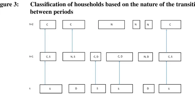
time periodt, so thatytis the average measure for the population in period t. We can divide our population (at timet) into two groups: those households that will turn out to survive to the next period (indicated with a superscriptS) and those that will dissolve at the end of the period (superscriptD). The corresponding average household outcome measures (e.g., household size) for those two subpopulations will be ySt and yDt . In the following period (i.e.,t+ 1), there will be households that have continued from the previous period (indicated with a superscriptC) and new households (superscriptN). The average outcome measures for those subpopulations can be written asyCt+1andyNt+1.
Figure 3 depicts our classification. Arrows connect the same households between periods. It is important to note that a continuing household in periodt+ 1can be either a ‘surviving’ or ‘dissolving’ one with respect to transitions to the following period. This is shown in the Figure by the fact that each household in periodt+ 1has both a C/N clas-sification as well as an S/D one. For the moment we are only interested in the transitions from periodttot+ 1. A household that will survive (from the perspective of periodt) has to be a household that has continued (from the perspective of periodt+ 1), soyC
t+1−ySt
is the change in the outcome measured on the same group of households, i.e.,
yCt+1−ySt = ∆ySt,t+1,
where the right hand side should be read as the change in the average value ofymeasured on the households that will be observed in bothtandt+ 1.
Figure 3: Classification of households based on the nature of the transitions between periods
The overall population averages in periodtandt+ 1can be written as weighted averages of the outcomes in their relevant subpopulations; i.e., we have
yt = (1−θt)yDt +θtySt
yt+1 = (1−φt+1)yNt+1+φt+1yCt+1,
whereθtis the proportion of households in periodtthat will survive to periodt+ 1and
φt+1 is the proportion of households in the population at timet+ 1that have survived from the previous period. In our diagramθt is 23 (four S households and two D ones),
whileφt+1is also23 (four C households and two N ones). So
∆yt+1=θt∆ySt,t+1+ (1−θt) yNt+1−y
D t
+ (θt−φt+1) yNt+1−y
C t+1
. (3) This decomposition is not unique. We could as easily have written
∆yt+1=φt+1∆ySt,t+1+ (1−φt+1) yNt+1−y
D t
+ (θt−φt+1) yDt −y S t
. (4) Unless there is a very rapid increase or decline in the number of householdsθt−φt+1 should be small and the two decompositions should give similar results. In the empirical results we report the first decomposition. The second provides qualitatively similar results and is available on request from the authors.
We term the three effects:
• The ‘within household change’ effectθt∆ySt,t+1
• The ‘replacement’ effect (1−θt) yNt+1−yDt
, since the difference yN t+1 −yDt
represents the effects of new households replacing those going out of existence
• The ‘dilution’ effect(θt−φt+1) yNt+1−y
C t+1
, sinceθt−φt+1is nonzero only if there is a net change in the number of households and the termyNt+1−yCt+1reflects how newly formed households differ from surviving ones. In a period of rapid household formation, the continuing (surviving) households become a decreasing fraction of the entire population of households. Their contribution to the overall mean household size therefore becomes diluted by the new households.
4. Data
4.1 Data requirements
A key requirement in order to implement this technique is an ability to identify house-holds that are the same in two time periods, so that we can measure∆yS
as households that are newly formed in any given period. Finally we need to be able to estimateθtandφt+1, the population proportions of households that will survive and
households that have continued, respectively.
Cross-sectional data will not allow us to estimate any of these quantities. However, demographic surveillance data and certain types of household panels will allow us to estimate all of these. We will discuss in turn these two types of data and the specific South African datasets that we will use.
4.2 Demographic surveillance data
Demographic surveillance sites have been set up in many countries in the world. The INDEPTH network (http://www.indepth-network.org) acts as umbrella organisation for many of them. Central to the operation of these sites is the monitoring of demographic events on a closed population on an ongoing basis. These sites therefore are well po-sitioned to track household formation and dissolution processes as well as the popula-tion proporpopula-tions required for the decomposipopula-tion. Many of these sites measure a range of household outcomes besides standard demographic variables for which the decomposi-tion would be suitable.
4.2.1 The Agincourt site
Figure 4: The original Agincourt field site covers 21 villages in the Bushbuckridge area
4.2.2 The Health and Demographic Surveillance System (HDSS)
The Agincourt HDSS monitors key demographic events and socioeconomic variables in the Agincourt sub-district. A baseline census was conducted in 1992 and since 1999 there have been annual census rounds (Kahn et al. 2012). The main demographic, health, and socioeconomic variables measured routinely by the HDSS include births, deaths, in-and out-migrations, household relationships, resident status, refugee status, education, and antenatal and delivery health-seeking practices (Tollman 1999; Tollman et al. 1999; Collinson et al. 2002). Temporary migrants are accounted for by including on the house-hold roster nonresident members who retain significant contact and links with the rural home (Collinson et al. 2001). The ‘share common pot’ definition of a household is thus expanded to include the temporary migrants who would normally share the same pot on return. The definition of household head is the main household decision maker, as re-ported by the household respondent. There have been several ‘add-on’ modules that have been run. For example every second year since 2000 there has been a household asset module which includes information on household access to services, e.g., electricity.
The software system used consists of a relational database constructed in Microsoft SQL Server.
4.2.3 Tracking households over time
One of the key questions for our empirical analysis is to identify the ‘same’ household at different time periods. The HDSS keeps track of dwelling units, households (linked to a ‘household head’ and to a dwelling), and individuals. For our purposes we have used the HDSS information to identify continuing households by:
• Dwelling: continuing residence in the same location
• Overlapping membership: there must be at least one individual from the previous household still living in the dwelling.
One of the implications of this definition is that if a family group moves from one dwelling to another (as a group) this will be classified as a household dissolution event followed by a household formation one. This definition was adopted partially for con-venience. Firstly, it corresponds to how the HDSS keeps track of households. Secondly, many of the moves of entire families are migrations out of the HDSS area. If we were to adopt a definition of the household that did not have a locational component, we would not know how to treat them in our analysis, since we don’t know what happened to them (they would be lost due to attrition). With our definition we do not need to know what happened to them because once the household has ‘dissolved’ it no longer features in any analyses.
While the locational definition is convenient, it also makes sense for our application. If one thinks about household services (provision of water, electricity), these are location-specific and it is useful to differentiate changes in access to a service for a given group of people at a location (a ‘household’) from changes induced by those people migrating to a different location.
4.3 Household panels
However, in subsequent waves information on the households in which those in-dividuals find themselves is also often recorded, leading in the case of the ECHP to a distinction between “sample and nonsample persons” (Peracchi 2002: 66). It is therefore possible, at least in principle, to classify households as surviving/newly formed/dissolving and to get estimates of household formation and dissolution rates. Harris (2016) has dis-cussed how this can be done for the South African household panel, the National Income Dynamics Study.
4.3.1 The National Income Dynamics Study (NIDS)
South Africa’s National Income Dynamics Study (NIDS) was modelled on other house-hold panels, such as the Panel Study of Income Dynamics in the United States (for more details see Leibbrandt, Woolard, and de Villiers 2009). It was commissioned by South Africa’s Presidency in an effort to track long-run poverty and well-being. The South-ern Africa Labour and Development Research Unit (SALDRU) at the University of Cape Town won the bid and ran the baseline study in 2008. Since then it has administered three other waves, around one round every second year. The core concerns of the study are incomes, expenditures, labour market participation, education, health (including anthro-pometrics), and household well-being (e.g., access to services).
At the baseline the sample was designed to be nationally representative. It was a two-stage sampling design with 400 primary sampling units (PSUs) extracted from Statistics South Africa’s 2003 master sample and a target of 24 households per PSU. The final realised sample was around 7,300 households and about 28,000 individuals Leibbrandt, Woolard, and de Villiers (2009). These individuals became the ‘Continuing Sample Members’ (CSMs) for the subsequent waves. Babies born to CSM women also became CSMs. At each of the subsequent waves, individuals who were coresident with CSMs were also interviewed. These individuals were classified as ‘Temporary Sample Members’ (TSMs).
4.3.2 Tracking households in NIDS
In order to implement our decomposition, we need to identify continuing households as well as newly formed and dissolving ones. We use the same decision rule as in the case of the Agincourt HDSS data; i.e., a household will be deemed to be the same if:
• it remains resident in the same location
• there is an overlap of membership from one period (wave) to the next.
sense given our application to household services. But making location central to the definition of the household is less self-evident in the case of NIDS than it is for the Ag-incourt HDSS, particularly since moves are tracked across South Africa. This raises the question whether choosing a different definition of a continuing household would change the results that we show below. For instance, we could define the ‘same’ household in two waves of NIDS by a ‘majority’ criterion – the successor household is that residential unit which contains more than 50% of the members of the current household, regardless of location. In the online appendix to this article, we outline this approach in more detail and show that it doesn’t affect the conclusions reached with the current definition. Differ-ent definitions have differDiffer-ent types of attrition and missing value problems. For instance with any of the definitions that we are using, we face a difficulty, if a single individual leaves one particular dwelling and is tracked to another one. We need to decide whether to identify that household as a newly formed one, or whether it should be thought of as an individual joining a existing household. This is of some importance, since pre-existing households (i.e., households that could have been sampled at baseline but were not) should not be included in the statistics when calculating wave-on-wave changes.
In order to differentiate between these for the case of our location-based definition, we use information on whether the TSMs in the household in question have also moved. If everyone has moved then it qualifies as a new household.
An additional problem is that if individuals are lost to the panel (i.e., the problem of attrition), we may also lose information about the fate of the households in which they reside; i.e., we may not know whether a particular household dissolved or continued (and if it continued what happened to the household outcome that we are interested in). This is potentially serious since household attrition is the most prevalent form of attrition in NIDS (Brown et al. 2012: 23). Around 16% of individuals could not be tracked from wave 1 to wave 2 because the entire household was lost from the sample – in most cases due to the fact that the household moved and could not be traced at the forwarded address. Another 2% attrited due to refusal to participate in the follow-up. As a result all analyses using NIDS (including cross-sectional ones) need to bear this in mind. In our analyses we see the same patterns in cross-sectional datasets which are not subject to attrition, and our longitudinal findings parallel those from Agincourt, which is not subject to this problem, so we are confident that our results are not an artefact of the missing data. Nevertheless, we still need to account for the attrition problem. There are at least three ways in which one might do this:
• reweight the observed observations for the ones lost to attrition
• impute outcomes to the attrited units
• bound the range of outcomes by assuming maximum or minimum values for the attrited units.
not (or whether the associated CSMs form new households), and have reweighted the observed units to account for any conditional attrition.
5. Methods
5.1 Changes in household size
We will investigate the usefulness of our decomposition technique in analysing the ob-served reduction in household size by three methods: Firstly, we will use the simple sectional evidence to track the changes over time. We will do so by using the cross-sectional components of both the Agincourt HDSS and the NIDS datasets, as well as the more standard nationally representative surveys run by Statistics South Africa: the Oc-tober Household Surveys, Labour Force Surveys, and Quarterly Labour Force Surveys. We will use the harmonised series of these datasets released as PALMS – postapartheid Labour Market Series (Kerr, Lam, and Wittenberg 2013). As noted by Kerr and Witten-berg (2015), however, the early household surveys provide biased evidence due to the undersampling of small households. Consequently we try to correct for that by weighting up the small households as discussed by Machemedze, Kerr, and Wittenberg (2014). We compare the sectional evidence from the national surveys to the equivalent cross-sectional pictures from the Agincourt HDSS data, and the NIDS data.
Secondly, we implement the Kuijsten decomposition technique given by equations 1 and 2 on all of the cross-sections available to us, viz. the Statistics SA household surveys as embodied in PALMS, the Agincourt HDSS, and NIDS.
Finally we implement our decomposition on the longitudinal data available in the Agincourt HDSS and NIDS.
5.2 Electricity connections
In the case of access to electricity we will also approach the topic incrementally, first using the available cross-sections to describe the changes, using the same type of survey evidence that we use in tracking household size, except that we make use of the General Household Surveys instead of the Labour Force Surveys.
We can provide a snapshot of how the roll-out of services proceeds by noting that the change in the count of unserviced households can be written as
H0,t
|{z}
unserviced HH att
+ (Ht+1−Ht)
| {z }
net new households
−(H1,t+1−H1,t)
| {z }
net new connections
= H0,t+1,
| {z }
where H1,t and H0,t refer to households with and without services respectively. By
dividing this identity byHtwe can express this in terms of rates
bt+rHHt,t+1−nt,t+1=b∗t+1, (5)
wherebtis the backlog in periodt, rtHH,t+1 is the household growth rate betweentand
t+ 1,nt,t+1 is the rate of new service connections andb∗t+1 is the backlog in period
t+ 1expressed as proportion ofHtrather thanHt+1. Of coursebt+1 =b∗t+1
Ht
Ht+1 =
b∗
t+1/ 1 +rtHH,t+1
, so it is easy to calculatebt+1givenbt,rtHH,t+1andnt,t+1. Equation 5
is useful because it expresses directly the implementation challenge facing government: the race between household formation and service roll-out and the impact this has on the evolution of the backlog.
In the final part of our analyses we implement the decomposition we outlined in sec-tion 3 on electricity connecsec-tions in the Agincourt HDSS and NIDS longitudinal datasets.
6. Results
6.1 Changes in household size
in average household size between 2008 and 2012, although the more restrictive definition shows an uptick in 2010.
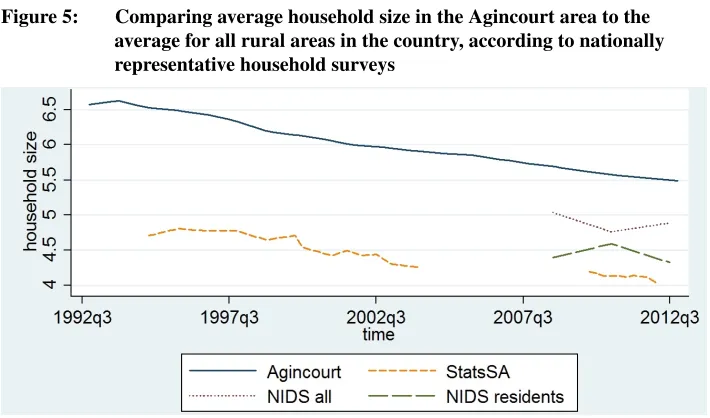
The effect of a less restrictive definition on the measurement of household size is also evident in the case of Agincourt, which also keeps migrant members on the household roster lists. Figure 5 presents the initial Agincourt picture. This is given by the solid line which shows a very smooth reduction of average household size over the period as a whole. This trend is juxtaposed with the ‘rural’ samples from the national surveys. From 2004 to 2008 there was no ‘rural’ indicator released with the LFSs, so there is a break in the overall trajectory in Figure 5. Nevertheless, it is evident that rural household size has also come down. The NIDS pattern is a bit more complicated, but it also suggests that over the period as a whole households became smaller.
Figure 5: Comparing average household size in the Agincourt area to the average for all rural areas in the country, according to nationally representative household surveys
Note: Own calculations from the following sources: Agincourt – Agincourt HDSS data. Stats SA – rural samples of October Household Surveys, Labour Force Surveys and Quarterly Labour Force Surveys, weights recalibrated for undersampling. NIDS all – rural sample from National Income Dynamics Study, all members. NIDS residents – as for NIDS, resident members only.
surveys includes some contexts which may better be thought of as periurban, whereas Agincourt is a ‘deep rural’ community.
Secondly the NIDS point estimates for 2010 seem somewhat odd: the gap between the looser and more restrictive definitions is much smaller in this period than in either 2008 or 2012. This suggests that the weighting corrections may not have properly cor-rected for selective attrition of certain types of households. This point is worth bearing in mind when assessing the decompositions below, in particular when analysing the changes from wave 1 to wave 2.
Thirdly, despite the differences in definitions and measurement, the magnitude of the reduction in household size over the period 1994 to 2012 is similar: around one person from an initial household size of 6.5 in the case of Agincourt and 0.7 from an initial household size of 4.7 in the case of the national surveys. Both amount to a 15% reduction.
Table 1: Change in the distribution of households
PALMS PALMS
Agincourt recalibrated original wts NIDS 1994–2012 1994–2012 1994–2012 2008–2012
Population growth rate (%) 22.1 26.0 26.0 5.5 Annual population growth (%) 1.1 1.3 1.3 1.3 Household growth rate (%) 45.1 51.0 59.2 9.9 Annual household growth (%) 2.1 2.3 2.6 2.4
Demographic effect 49.0 50.9 43.9 55.5
Structure effects
1-person households 11.1 31.0 40.0 83.4 2-person households 10.1 13.9 18.0 –15.7 3-person households 16.3 13.3 10.0 –17.1 4-person households 16.3 8.0 5.2 –17.2 5-person households 10.4 –1.2 –2.1 1.2 6-person households 5.4 –3.1 –3.2 2.9 7-person households –1.1 –4.5 –4.2 3.3 8-person households 0.0 –2.9 –2.7 1.1 9-person households –3.6 –2.0 –1.8 4.6 10-person households –3.2 –3.6 –3.4 –0.2 11-person households –2.4 0.4 0.4 –1.5 12-person households –1.7 0.1 0.1 2.1 13-person households –1.1 0.0 0.0 –1.2 14-person households –0.5 0.0 0.0 0.5 15+-person households –4.7 –0.1 –0.1 –1.7
pop-ulation growth rate: ranging from an average of 2.1% per annum in the case of Agincourt to 2.6% per annum if the Statistics SA datasets are used with the unadjusted weights. As we argued earlier, there is good evidence to suggest that the early OHSs undersampled small households and as a result underestimated the total number of households. The recalibrated estimates suggest a growth rate of 2.3% for the number of households.
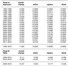
Table 2: Decomposing change in household size
Panel A: overall
Agincourt change within replace dilute
1994–1995 –0.036 0.0456 –0.0309 –0.0507 1995–1996 –0.059 –0.0054 –0.0271 –0.0267 1996–1997 –0.093 0.0394 –0.0717 –0.0603 1997–1998 –0.141 0.0000 –0.1170 –0.0242 1998–1999 –0.050 0.0595 –0.0096 –0.1003 1999–2000 –0.067 0.0207 –0.0461 –0.0421 2000–2001 –0.081 –0.0232 –0.0069 –0.0511 2001–2002 –0.032 –0.0125 –0.0026 –0.0172 2002–2003 –0.046 –0.0238 0.0043 –0.0263 2003–2004 –0.042 –0.0194 0.0087 –0.0310 2004–2005 –0.022 0.0026 0.0036 –0.0280 2005–2006 –0.064 –0.0145 0.0066 –0.0558 2006–2007 –0.060 –0.0297 0.0172 –0.0479 2007–2008 –0.056 –0.0085 0.0105 –0.0582 2008–2009 –0.062 –0.0199 0.0213 –0.0637 2009–2010 –0.047 –0.0004 0.0087 –0.0552 2010–2011 –0.044 0.0101 0.0072 –0.0618 2011–2012 –0.032 0.0144 0.0033 –0.0497
1994–2012 –1.034 0.0350 –0.2205 –0.8502
Panel B: overall
NDIS change within replace dilute
2008–2010 0.111 0.236 –0.064 –0.062 2010–2012 –0.248 –0.032 –0.113 –0.140
2008–2012 –0.137 0.204 –0.177 –0.202
might have expected to have been particularly hard to track. With the exception of the NIDS results, the structure effects suggest a clear shift in the distribution of household types from bigger to smaller households. On its own, however, this does not indicate what happened ‘within’ households.
The results from our decomposition are given in Table 2. The decomposition for the Agincourt demographic data is given in the top panel. It indicates that over the period 1994 to 2012 households shed (on average) one member. Interestingly, however, none of this happened ‘within’ continuing households. If anything, continuing households grew a tiny amount (0.035). Around 21% of the reduction is accounted for by the fact that newly formed households were smaller than dissolving households. The balance is due to the dilution effect – the fact that there were so many new households, significantly smaller than the continuing ones, that they managed to bring down the overall average household size by 0.85 persons over this period. It is clear that these new households on the whole did not emerge as ‘break-aways’ from existing households, since there is no evidence that these became smaller. Instead it seems that household dissolution (in this context often migration events) are key episodes leading to the reconstitution of households.
The NIDS panel covers a much shorter time period, but it provides the same take-home message. We see (in Panel B of Table 2) that the ‘replacement’ and ‘dilution’ effects are again strongly negative. In this case, however, they are somewhat offset by growth within continuing households between wave 1 and wave 2. It again seems clear that household dissolution, reconstitution, and rapid new household formation are the key drivers of the observed decrease in household size.
6.2 Changes in household energy connections
Figure 6: Penetration of household electricity use in the Agincourt area
according to two measures: household electricity uses for lighting and cooking
Table 3 provides evidence how important the interplay between household dynamics and connection rates are. We see in the top part of the panel that over the 18-year period covered by the General Household Surveys and October Household Surveys, the number of households using electricity for lighting increased around 160%. This translates into an annual increase in connections of more than 5%. The Agincourt data on infrastructure is for a shorter time period, but over the ten years between 2001 and 2011 additional connections also increased at more than 5% per annum. These rates of increase are in line with the rapid electrification documented by Gaunt (2005).
Table 3: Change in the availability of electricity
OHS/GHS OHS/GHS
Agincourt recalibrated original NIDS 1994–2012 1994–2012 1994–2012 2008–2012
Growth in connections (%) 72.2 156.9 169.3 17.3 Annual growth rate in connections (%) 5.58 5.38 5.66 4.07 Population growth (%) 12.21 23.79 23.50 5.48
Change in backlog
This rapid rate of service roll-out, however, occurred against a backdrop of rapid household formation, as we noted in the previous section. Compared to the baseline backlog of 31% of households in the Agincourt area in 2001 the new connection rate of 50% would have more than wiped out the backlog, if it hadn’t been for the fact that new household formation added 26% on to the baseline. Nevertheless, the roll-out was sufficiently strong that it brought the overall backlog down to 6% at the end of the period. The same pattern can be seen in the case of the national data for the period 1994 to 2012. We see that whether or not we recalibrate the OHSs to take account of the deficit of small households, the new connection rate would have entirely eliminated the national backlog if it hadn’t been for new households being formed. The only period in which this does not seem to have been the case is the period since 2008, as measured by the National Income Dynamics Study. Nevertheless, even in this case new connections outstripped new households thus ensuring that the overall backlog came down.
Table 3 also provides the population growth rate over the period covered by the data. If household formation had been at this lower rate, then a simple counterfactual calculation suggests that the new connection rate would have been sufficient to eliminate the entire backlog in the case of both Agincourt and the country as a whole for the period 1994 to 2012.
The cross-sectional picture therefore strongly points to the importance of the con-nection between net household formation dynamics and the evolution of the proportion of households with services. Table 4 shows how these dynamics play themselves out on the ‘intensive’ and ‘extensive’ margin, in terms of our households’ decompositions.
Table 4: Decomposing change in electricity availability
Panel A: overall
Agincourt change within replace dilute
2001–2003 0.075 0.0782 0.0087 –0.0119 2003–2005 0.130 0.1220 0.0063 0.0015 2005–2007 –0.011 –0.0036 0.0022 –0.0096 2007–2009 0.051 0.0633 0.0019 –0.0146 2009–2011 0.005 0.0086 –0.0128 0.0094
2001–2011 0.250 0.2686 0.0063 –0.0252
Panel B: overall
NDIS change within replace dilute
2008–2010 –0.020 0.009 –0.011 –0.001 2010–2012 0.077 0.058 0.019 0.002
The pattern for Agincourt, shown at the top of the table, is clear-cut. The 25-percentage-point increase in services (and an equivalent drop in the backlog) occurred entirely ‘within’ households; i.e., households did not improve their access by moving to a serviced location, but received new connections at their current location. Indeed the ‘di-lution’ effect is negative, suggesting that newly formed households had less access than continuing households. In fact the differenceyN
t+1−yCt+1is0.189 when averaged across the five data points. This suggests that families move to locations that are initially unser-viced, but that over time acquire services. The fact that the ‘replacement’ effect is weakly positive suggests that households that dissolve/migrate had even worse access than the newly formed households.
The pattern in the NIDS dataset is more complicated. The 2008 to 2010 changes suggest that the drop in access (shown in Figure 2) is mainly driven by loss of access within continuing households, but that dissolving households also had better access than new ones (leading to a negative ‘replacement’ effect). This is an interesting observation since it raises the possibility that in some instances roll-out of services has occurred in areas which may lose population in subsequent periods. Interestingly enough the Agin-court area also showed a negative replacement effect in this period (2009–2011). This possibility is important for policy purposes, since it means that planning of electrifica-tion, as discussed, for instance by Bekker et al. (2008) needs to be aware of not only the rate at which household growth is likely to outstrip population growth, but also migration patterns.
In the case of NIDS, the transitions from 2010 to 2012 show reversals in the signs of both of these effects. In neither period does dilution seem to change aggregate connection rates much.
The negative ‘within’ effects in NIDS 2008–2010 and in Agincourt 2005–2007 are of some interest because they indicate that the net increase in connections shown in the aggregate statistics in Table 3 may actually conceal some disconnections. Harris (2016) has investigated these in the NIDS data in more detail. What was driving these is a topic for future research.
7. Conclusion: Households and social dynamics
The central concern of the paper has been to reflect on some of the big changes that have occurred in the nature of households and in the access to household services over the postapartheid period. The statistics shown in table 1 show a very rapid rate of household formation and a shift towards smaller households. In table 3 we have shown that the roll-out of electricity has been even more rapid than net household formation. These rates are truly impressive and provide the background for any research that is trying to understand how this occurred.
We argue that any analysis of households and household services has to grapple with the fact that households are not fixed entities, as much of the existing literature has as-sumed, but are subject to recomposition, dissolution, and re-formation. Changes happen both ‘within’ households and at the dissolution/formation margin. Our decomposition draws specific attention to these. In the case of changes in household size we showed that much of the change seems to occur at the point where people leave one location and then set up at another. In a few cases these dissolution/formation processes also have im-plications for service access. More commonly, however, the rapid process of household formation sets up a ‘race’ in which the roll-out of services is continually trying to play catch-up with newly set up less-serviced households. Our decompositions manage to draw attention to these processes. Our decompositions have also revealed that the service roll-out is not always a linear process: Disconnections seem to occur also and in some cases households seem to leave dwellings with services in favour of locations without them. This has not been noted hitherto.
Even so, our decomposition relies on averages which smooth over new connections and disconnections. It is therefore not the last word on the full complexity of household changes. For that other tools will be necessary, e.g., some of the more conventional panel techniques. Nevertheless, even in those cases it is worth taking note of the fact that many interesting changes happen not within the panel, but at the point at which entities exit and enter.
8. Acknowledgements
References
Amoateng, A. (2007). Towards a conceptual framework for families and households. In: Amoateng, A. and Heaton, T. (eds.).Families and households in post-apartheid South Africa: Socio-demographic perspectives. Cape Town: HSRC Press: 27–42.
Amoateng, A. and Heaton, T. (2007). Families and households in post-apartheid South Africa: Socio-demographic perspectives. Cape Town: HSRC Press.
Amoateng, A., Heaton, T., and Kalule-Sabiti, I. (2007). Living arrangements in South Africa. In: Amoateng, A. and Heaton, T. (eds.).Families and households in post-apartheid South Africa: Socio-demographic perspectives. Cape Town: HSRC Press: 43–59.
Amoateng, A. and Kalule-Sabiti, I. (2008). Socio-economic correlates of the incidence of extended household living in South Africa. Southern African Journal of Demography
11(1): 75–102.
Amoateng, A. and Richter, L. (2007). Social and economic context of families and house-holds in South Africa. In: Amoateng, A. and Heaton, T. (eds.).Families and house-holds in post-apartheid South Africa: Socio-demographic perspectives. Cape Town: HSRC Press: 1–25.
Bekker, B., Eberhard, A., Gaunt, T., and Marquard, A. (2008). South Africa’s rapid electrification programme: Policy, institutional, planning, financing and technical in-novations. Energy Policy36(8): 3125–3127.doi:10.1016/j.enpol.2008.04.014. Bhorat, H. and van der Westhuizen, C. (2013). Non-monetary dimensions of well-being
in South Africa, 1993–2004: A post-apartheid dividend?Development Southern Africa
30(3): 295–314. doi:10.1080/0376835X.2013.817308.
Brown, M., Daniels, R., Villiers, L., Leibbrandt, M., and Woolard, I. (2012). National Income Dynamics Study Wave 2 user manual. Cape Town: Southern Africa Labour and Development Research Unit.
Casale, D., Muller, C., and Posel, D. (2004). ‘Two million net new jobs:’ A reconsidera-tion of the rise in employment in South Africa: 1995–2003. South African Journal of Economics72(5): 978–1002.doi:10.1111/j.1813-6982.2004.tb00141.x.
Collinson, M., Mokoena, O., Mgiba, N., Kahn, K., Tollman, S., Garenne, M., Herbst, K., Malomane, E., and Shackleton, S. (2002). Agincourt DSS, South Africa. In:
Populations and their health in developing countries, Volume 1: Population, health and survival at INDEPTH sites. Ottawa: IDRC Press: 197–206.
of the Witwatersrand. (Agincourt Health and Population Unit working paper).
Dinkelman, T. (2011). The effects of rural electrification on employment: New evidence from South Africa. American Economic Review101(7): 3078–3108. doi:10.1257/aer. 101.7.3078.
Gaunt, C. (2005). Meeting electrification’s social objectives in South Africa, and im-plications for developing countries. Energy Policy33(10): 1309–1317. doi:10.1016/ j.enpol.2003.12.007.
Harris, T. (2016). Household electricity access and household dynamics. [Master’s dis-sertation]. Cape Town: School of Economics, University of Cape Town.
Hosegood, V., Benzler, J., and Solarsh, G. (2005). Population mobility and household dynamics in rural South Africa: Implications for demographic and health research.
Southern African Journal of Demography10(1/2): 43–68.
Hundenborn, J., Leibbrandt, M., and Woolard, I. (2016). Drivers of inequality in South Africa. Cape Town: Southern African Labour and Development Research Unit. (SAL-DRU working paper 194).
Kahn, K., Collinson, M., G´omez-Oliv´e, F., Mokoena, O., Twine, R., Mee, P., Afolabi, S., Clark, B., Kabudula, C., Khosa, A., Khoza, S., Shabangu, M., Silaule, B., Tibane, J., Wagner, R., Garenne, M., Clark, S., and Tollman, S. (2012). Profile: Agincourt Health and Socio-demographic Surveillance System. International Journal Of Epidemiology
41(4): 988–1001.doi:10.1093/ije/dys115.
Kerr, A., Lam, D., and Wittenberg, M. (2013). Post-Apartheid Labour Market Se-ries 1994–2012, version 2.1 [dataset]. [electronic resource]. Cape Town: DataFirst.
http://www.datafirst.uct.ac.za/catalogue3/index.php/catalog/434.
Kerr, A. and Wittenberg, M. (2015). Sampling methodology and field work changes in the October Household Surveys and Labour Force Surveys. Development Southern Africa32(5): 603–612. doi:10.1080/0376835X.2015.1044079.
Kuijsten, A. (1995). Recent trends in household and family structures in Europe: An overview. In: van Imhoff, E., Kuijsten, A., Hooimeijer, P., and van Wissen, L. (eds.).Household demography and household modeling. New York: Plenum: 53–84.
doi:10.1007/978-1-4757-5424-7 3.
Leibbrandt, M., Finn, A., and Woolard, I. (2012). Describing and decomposing post-apartheid income inequality in South Africa.Development Southern Africa29(1): 19– 34.doi:10.1080/0376835X.2012.645639.
Study. (Technical paper 1).
Leibbrandt, M., Woolard, I., Finn, A., and Argent, J. (2010). Trends in South African income distribution and poverty since the fall of Apartheid. Paris: OECD Publishing. (OECD Social, Employment and Migration working papers 101).
Machemedze, T., Kerr, A., and Wittenberg, M. (2014). Recalibrating the OHSs to adjust for sampling changes. Cape Town: University of Cape Town, DataFirst. (Technical paper 28).
Niehaus, I. (2001). Witchcraft, power and politics: Exploring the occult in the South African Lowveld. London: Pluto Press.
Peracchi, F. (2002). The European Community Household panel: A review. Empirical Economics27(1): 63–90. doi:10.1007/s181-002-8359-0.
Posel, D., Fairburn, J., and Lund, F. (2006). Labour migration and households: A re-consideration of the effects of the social pension on labour supply in South Africa.
Economic Modelling23: 836–853.doi:10.1016/j.econmod.2005.10.010.
Rose, D. (1995). Household panel studies: An overview. Innovation: The European Journal of Social Sciences8(1): 7–24.
Russell, M. (2003a). Are urban black families nuclear? A comparative study of black and white South African family norms. Social Dynamics29(2): 153–176. doi:10.1080/ 02533950308628679.
Russell, M. (2003b). Understanding Black households: The problem. Social Dynamics
29(2): 5–47.doi:10.1080/02533950308628674.
Schatz, E., Madhavan, S., Collinson, M., G´omez-Oliv´e, X., and Ralston, M. (2015). Dependent or productive? A new approach to understanding the social positioning of older South Africans through living arrangements.Research on Aging37(6): 581–605.
doi:10.1177/0164027514545976.
Tollman, S. (1999). The Agincourt field site: Evolution and current status.South African Journal of Medicine89(8): 855–857.
Tollman, S., Herbst, K., Garenne, M., Gear, J., and Kahn, K. (1999). The Agincourt demographic and health study: Site description, baseline findings and implications.
South African Journal of Medicine89(8): 858–864.
Udjo, E. (2015). Projecting population, numbers of households and dwelling units in South Africa 2011–2021.African Population Studies29(1): 1510–1524.doi:10.11564/ 29-1-698.
Africa, 1996–2003. Scandinavian Journal of Public Health35(Suppl. 69): 130–137.
doi:10.1080/14034950701355429.