Improving Pairwise Preference Mining Algorithms Using
Preference Degrees
Juliete A. Ramos Costa, Sandra de Amo
Federal University of Uberlˆandia-MG, Brazil [email protected], [email protected]
Abstract. Different preference mining techniques designed to predict a preference order on objects have been proposed in the literature, with very good accuracy results. In this article, we propose to consider not only the fact that the user prefer an itemi1to an itemi2 but also the degree of his preference on the two items. We propose the algorithm FuzzyPrefMiner designed to predict fuzzy preferences and show through a series of experiments that it outperforms pairwise preference mining techniques whose training phase do not include information on preference degrees.
Categories and Subject Descriptors: H.2.8 [Database Management]: Database Applications—data mining; I.2.6 [Artificial Intelligence]: Learning—concept learning
Keywords: data mining, fuzzy preference, preference mining
1. INTRODUCTION
Most known recommendation systems, following a collaborative filtering or a content-based approach, rely on explicit user preference feedback data in order to provide recommendations on items not yet seen by the user. These explicit preference data are given by theutility matrix which contains at each positioni, j the rating given by userito itemj. However, this explicit way to get user feedback lacks of effectiveness, since most users are unwilling to rate items while browsing the web. Moreover, the information obtained in that way may be biased, since it does not include preferences from users who are not keen on rating things. Another drawback of using explicit user feedback is related to the fact that the rating scale is fixed (normally going from 0 to N, where N is the maximum rating permitted). Let us suppose that a userurated a movie f1 asN since he/she loved it. Sometime later usaw the movief2 which he/she liked more thanf1. In this case, since past given ratings cannot be modified,
uis forced to give equal ratings (namely N) to both movies, even iff2 is largely preferred tof1.
For those reasons, we argue that preference data obtained in an implicit manner (by inferring user preferences from his/her browsing behavior) and following a pairwise representation (the user preference is represented by a set of pairs of items (i1, i2) telling thati1 is preferred toi2) are more desirable. For instance, let us suppose that, while browsing the IMDB website1, user u spent 30 seconds on the page of movief1 and 10 minutes on the page off2. One can infer that uis far more interested on filmf2than on filmf1. One can go a step further and assume thatuprefersf2tof1and represent this preference as a pair (f2, f1). Pairwise preference data obtained in this implicit way do not contain sufficient information for inferringspecific ratings on items. However, they are sufficient for inferring aranking of the top-k films the user would probably like, and consequently, recommend those films to him/her [Cohen et al. 1999].
1www.imdb.com
Most preference mining methods proposed in the literature rely on explicit ratings provided by the user as input data represented by means of ascore function [Cohen et al. 1999; Crammer and Singer 2001; Burges et al. 2005]. Pairwise representation [Jiang et al. 2008; Koriche and Zanuttini 2010; de Amo et al. 2013; de Amo et al. 2012] andRanking2representation [Joachims 2002; Freund et al. 2003] are receiving more attention in recent research.
Preference mining techniques that use input data following a pairwise representation usually obtain this input data directly from the user, using a pre-processing step for transforming explicit user rating into pairs3. For instance, if the user evaluated itemi
1as 5 andi2as 1, this information is transformed into the pair (i1, i2). We claim that in this transformation, a lot of information has been lost. Indeed, if the ratings were 5 and 4, the same pair (i1, i2) would be obtained. In the first situation, the user prefers objecti1to i2more intensely than in the second situation.
In previous work [de Amo et al. 2013] we proposed the algorithm CPrefMiner for mining acrisp contextual preference model from a set of preference samples represented as pairs of alternatives. The model is said to becrisp since the input data provided by the user is based on yes/no alternatives (either he/she prefers objecti1 to objecti2or vice-versa) and the output model allows to predict if a new objecti3is preferred to a new object i4 or vice-versa. The mined preference model is said to be contextual since it is constituted by a set ofcontextual preference rules [Wilson 2004] of the form IF
<context>then I prefer ‘this’ to ‘that’. For instance: For films directed by Spielberg, I prefer Action to Comedy whereas for films directed by Woody Allen I prefer Comedy to Action. The preference model extracted by CPrefMiner is capable to infer anorder relation on objects(a task that a classifier would not be able to achieve!), that is, it is capable to infertransitivity relationships (if i1 i2 and
i2i3theni1i3 4) and also satisfyingirreflexibility (i16i1).
The main hypothesis of this article is that“the more information is enclosed in the input preference data, the more efficient is the mined preference model”. We propose the method FuzzyPrefMiner to mine fuzzy contextual preference model from a set of preferences samples represented as triples (i1, i2, n) wherei1andi2are items evaluated by a useruandnis thedegree of preference(0≤n≤1) of i1 w.r.t. i2 provided by user u. An extensive set of experiments comparing CPrefMiner and FuzzyPrefMiner validates this hypothesis: FuzzyPrefMiner is far more accurate then CPrefMiner to predict user preferences. Besides, the preference knowledge extracted by FuzzyPrefMiner is more refined then the one provided by CPrefMiner, since it is capable to predict not only ifi1i2 but also the degree of preference ofi1with respect toi2. We present in this article a subset of the experiments carried out to validate our hypothesis.
Fuzzy preference modeling and reasoning has been extensively studied in the last decade [Chiclana et al. 1998; Herrera-Viedma et al. 2004; Ma et al. 2006; Xu et al. 2013]. However, to the best of our knowledge this kind of preference model has not yet been exploited in the preference mining research.
2. PROBLEM FORMALIZATION
In this section, we formalize the problem of mining fuzzy contextual preferences, introducing the notion offuzzy preference model (FPM), how it is used to order things and some quality measures to evaluate its order predicting capability.
AFuzzy Preference Relation over a set of objects X ={x1, ..., xn} is a n×nmatrix P such that
Pij ∈ [0,1] represents the degree of preference (dp) of u over objects xi and xj. Fuzzy preference
relations have been introduced in Chiclana et al. [1998] and should satisfy certain conditions (see
2The user provides a sequence of objects in decreasing order of preference.
3Notice that, as argued before, pairwise preference data could also be obtained indirectly by examining the user’s
browsing behavior.
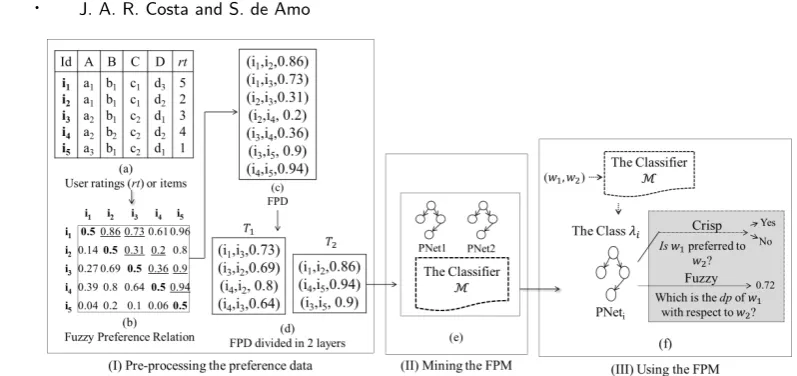
Fig. 1. Fuzzy Contextual Preference Mining Process.
Chiclana et al. [1998] for details), the most important being the reciprocity property Pij = 1−Pji
(which entails that Pii = 0.5). One way of obtaining fuzzy preference relations from a set of item
ratings provided by the user is to considerPij =f(rrji), whereriis the ratinguassigned to itemxiand
f is a function belonging to the family{fn:n≥1},fn(x) = x
n
xn+1. This family of functions produces
matrices satisfying all the properties required for fuzzy preference relations. Fig. 1(b) illustrates the fuzzy preference relation corresponding to the item-rating database of Fig. 1(a). Here, functionf2 has been considered forfuzzification.
AFuzzy Preference Database (FPD)over a relation schemaR(A1, ..., An) is a finite setP ⊆Tup(R)
× Tup(R) × [0,1] which is consistent, that is, if (i, j, n) ∈ P and (j, i, m) ∈ P then m = 1−n. The triple (i, j, n) represents the fact that the user prefers the tuple i to the tuple j with a degree of preference n. Fig. 1(c) illustrates a fuzzy preference database corresponding to a subset of the information contained in the matrix depicted in Fig. 1(b) (the triples presented in (c) correspond to the underlined positions of (b)).
Pre-processing the FPD: Let P be a fuzzy preference database. First of all, triples with dp < 0.5 are transformed into triples with dp ≥ 0.5. For instance, triple (i2, i3,0.31) in Fig. 1(c) becomes (i3, i2,0.69). After doing that, letdpmin(resp. dpmax) be the smallest (resp. the largest)dpappearing
in (the transformed)P.
Partition of P into k layers: First, let us partition the intervalI= [dpmin, dpmax] intokdisjoints and
contiguous subintervals I1, ..., Ik, such thatS k
i=1Ii =I. Second, partition P into k disjoint subsets
of triplesP1,...,Pk. EachPi is obtained by inserting intoPiall triples (w1, w2, n) withn≥0.5 such that (w1, w2, n) or (w2, w1,1−n)∈ P. Fig. 1(d) illustrates this step.
Layers can be viewed as classes: Let Ii = [ai, bi] and λi = ai+2bi. Triples (w1, w2, n) in Ii are
characterized by tuplesw1 andw2 having an average “intensity” of preferenceλi between them. For
instance, triples of layerT1 in Fig. 1(d) are associated to classλ1 = 0.72 (average of 0.73, 0.69, 0.8 and 0.64).
The Fuzzy Preference Model (FPM): The fuzzy preference model proposed in this article is a
structureFk =<M,P N et1,...,P N etk>, whereMis a classification model extracted from the set of
layers I1, ..., Ik (considering elements inIi as (w1, w2, λi) with the extra “class” dimension λi), and
P N eti is a Bayesian Preference Network (BPN) extracted from layer Ii, for all i = 1, ..., k. BPNs
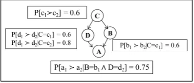
Fig. 2. A Bayesian Preference Network.
mine several BPNs, one for each layer. Fig. 1(e) illustrates a FPM extracted from the pre-processed preference input data of Fig. 1(d). BPNs are defined as follows:
Definition 2.1 [de Amo et al. 2013]. ABayesian Preference Network(BPN) over a relational schema R(A1, ..., An), consists in: (1) a directed acyclic graph Gwhose nodes are attributes in{A1, ..., An}
and the edges stand forattribute dependency and (2) a mapping θ that associates to each node ofG
a finite set of conditional probabilities (see Fig. 2).
Fig. 2 illustrates a BPN PNet1 over the relational schema R(A, B, C, D). Notice that, the pref-erence on values for attribute Bdepends on the context C: if C =c1, the probability that value b1 is preferred to valueb2 for the attributeB is 60%. The following example illustrates how BPNs are used to predict the order between two new tuples in the crisp scenario:
Example 1: Let us consider the BPN PNet1 depicted in Fig. 2. In order to compare two new tuples w1 = (a1, b1,c1,d1) and w2 = (a2, b2,c1,d2), we proceed as follows: (1) Let ∆(w1, w2) be the set of attributes for which w1 and w2 differ. In this example, ∆(w1, w2) = {A, B, D}; (2) Let min(∆(w1, w2))⊆∆(w1, w2) such that the attributes in min(∆) have no ancestors in ∆ (according to graphGunderlying the BPNPNet1). In this example, min(∆(w1, w2)) ={D,B}. The necessary and sufficient conditions forw1to be preferred tow2are: w1[D]w2[D] andw1[B]w2[B]; (3) Compute the following probabilities: p1 = probability thatw1w2 =P[d1 d2|C=c1]∗P[b1b2|C =c1] = 0.6 * 0.6 = 0.36;p2 = probability thatw2> w1 =P[d2 d1|C =c1]∗P[b2b1|C=c1] = 0.4 * 0.4 = 0.16. In order to comparew1 andw2 we select the highest betweenp1 andp2. In this example,
p1 > p2 and so, we infer that w1 is preferred to w2. If p1 = p2, a random choice decides if w1 is preferred tow2 or vice-versa. So, a BPN is capable to compare any pair of tuples: either iteffectively infer the preference ordering without randomness or it makes a random choice.
How a FPM can be used to predict preference degree between tuples: Let Fk =
<M,P N et1,...,P N etk>be ak-layer FPM and let w1,w2 be two new tuples. First of all, we have to infer the intensity of preference between these tuples. The classifierMis responsible for this task: it is executed on (w1, w2) and returns a classλi for this pair. Then the BPNP N eti,specific for this
layer, is executed on (w1, w2) to decide which one is preferred. This execution follows the same steps as illustrated inExample 1. IfP N etidecides thatw1 is preferred tow2 (resp. w2is preferred tow1), the final prediction is: w1is preferred to w2 with degree of preferenceλi (resp. 1−λi). Remark that,
the classifierMonly decides how intense the preference between the tuples is. The BPN decides the preference orderingbetween them. This prediction may beeffective orrandomas remarked at the end ofExample 1. Fig. 1(f) shows how a FPM can be used to predict both crisp and fuzzy preferences.
Measuring the quality of a fuzzy preference model: Since an exact match between the
pre-dicteddp (dpp) and the real one (dpr) is quite unlikely to occur, we consider a threshold σ > 0 to
measure how good is the prediction. We consider that the predicted dpp is correct if the following
conditions are both verified: (1)|dpr−dpp|≤σand (2) (dpr≥0.5 anddpp≥0.5) or (dpr<0.5 and
dpp <0.5). We say that the inference is effective (resp. random) depending on the effectiveness or
measures on atest FPDP:
The Accuracy(acc): defined by acc(Fk,P,σ)=NeM+Nr, where M is the number of triples in P, Ne
(resp. Nr) is the amount of triples (t1, t2, dpr) ∈ P for which thedpp inferred by Fk is effectively
(resp. randomly) correct;
TheRecall(rec): defined byrec(Fk,P,σ)= NMe;
TheRandomness Rate(rr): defined byrr(Fk,P,σ)= NMr;
ThePrecision(prec): defined byprec(Fk,P,σ)= NNec, where Nc is the number of triples (t1, t2, dpr)
∈ P that have been effectively compared byFk (correctly or not);
TheComparability Rate(cr): defined byrec(Fk,P,σ))= NMc.
Example 2: Let us consider tuplesw1andw2ofExample 1. Let us also suppose the input FPD depicted in Fig. 1(d) with its 2-layer partitionsT1 andT2. The corresponding classes areλ1 = 0.72 (average
dpof [0.64, 0.8]) and λ2 = 0.865 (averagedp of [0.83, 0.9]). Let us suppose thatdpr(w1, w2) = 0.76 and that the classifierMassigns the classλ1to (w1, w2). Notice that, the classifier only predicts that the intensity of preference between the two tuples is 0.72. It doesn’t say anything about theordering of preference between them. This task is achieved by the BPN1 associated to partition T1. Let us suppose that BPN1is the same as the one illustrated in Fig. 2. It comparesw1andw2as described in Example 1, by calculating the probabilitiesp1= 0.36 andp2= 0.16. Asp1> p2then the predicteddp isdpp=λ1= 0.72. So, both dpr anddpp are≥0.5 (condition (2) of the quality test is verified). Let
us consider parameterσ= 0.05 as in the experiments of Section 5. Since|0.76−0.72|= 0.04<0.05, we conclude that the fuzzy model correctly and effectively predicted thedpofw1 w.r.t. w2.
The Problem of Mining Fuzzy Contextual Preferences: This problem consists in, given a fuzzy
preference database andk >0, return ak-layer fuzzy preference modelFk having good quality with
respect toacc, prec, rec, crandrrmeasures and a given threshold σ.
3. ALGORITHM FUZZYPREFMINER
The FuzzyPrefMiner algorithm we propose to solve the Fuzzy Contextual Preference Mining Problem follows the same strategy of the algorithm CPrefMiner proposed in de Amo et al. [2013] to solve the crisp counterpart problem. The general framework of the algorithm is showed in Alg. 1. In this section, we present the details only of the parts of the method that have been modified in order to treat the fuzzy information. The specific procedures which have been modified are indicated inside a rectangle, in boldface.
3.1 Learning the Network Structure
ProcedureExtract(Alg. 2)[de Amo et al. 2013] is responsible for learning the network topologyGfrom the training preference databaseP. Gis a graph with vertices in A1, ..., An. An edge (Ai, Aj) in G
Algorithm 1:The FuzzyPrefMiner Algorithm
Input: A Fuzzy Preference DatabasePiover relational schemaR(A1, ..., An) %corresponding to a layer in the
entire training FPDP; Output: A BPNPNet
1 Extract(P,G);
2 foreachi= 1, . . . , ndo
3 Parents(G, Ai) = [Ai1, ..., Aim];
4 CPTable(Ai, Parents(Ai, G))=[CP rob1, ..., CP robl] ;
Algorithm 2:Extract Procedure
Input:P: a fuzzy preference database over relational schemaR(A1, ..., An);β: population size;ϑ: number of generations;γ: number of attribute orderings
Output: A directed graphG= (V, E), with verticesV ⊆ {A1, ..., An}that fits best to the fitness function
1 foreachi= 1, . . . , γdo
2 Randomly generate an attribute ordering;
3 Generate an initial populationI0of random individuals;
4 Evaluate individuals inI0, i.e., calculate their fitness ;
5 foreachj-th generation,j= 1, . . . , ϑdo
6 Selectβ/2 pairs of individuals fromIj;
7 Apply crossover operator for each pair, generating an offspring populationIj0;
8 Evaluate individuals ofI0
j;
9 Apply mutation operator over individuals fromI0j, and evaluate mutated ones;
10 FromIj∪Ij0, select theβfittest individuals through an elitism procedure;
11 Pick up the best individual after the last generation;
12 returnthe best individual among allγGA executions
means that the preference on values for attributeAj depends on values of attributeAi. That is,Aiis
part of the context for preferences over the attributeAj. This learning task is performed by a genetic
algorithm which generates an initial populationPof graphs with vertices inA1, ..., An and for each
graphG ∈Pevaluates a fitness functionscore onG. Full details on the codification of individuals and on the crossover and mutation operations are presented in de Amo et al. [2013].
The Fitness Function. This is the only part of theExtractprocedure where the degrees of preference included in the input data are relevant. The degree of preference affects primarily the way one decides if a given structure is good or not.
The main idea of the fitness function is to assign a real number (a score) in [−1,1] for a candidate structureG, aiming to estimate how good it captures the dependencies between attributes in a fuzzy preference databaseP. In this sense, each network arc is “punished” or “rewarded”, according to the matching between each arc (X, Y) inGand the correspondingdegree of dependenceof the pair (X, Y) with respect toP (see Alg. 3).
Thedegree of dependence of a pair of attributes (X, Y) with respect to a FPD P is a real num-ber that estimates how preferences on values for the attribute Y are influenced by values for the attribute X. Its computation is carried out as described in Alg. 3. In order to facilitate the description of Alg. 3, we introduce some notations as follows: (1) For each y, y0 ∈ dom(Y),
y 6= y0 we denote by Tyy0 the subset of pairs (t, t0) ∈ P, such that t[Y] = y ∧t0[Y] = y0 or t[Y] = y0 ∧t0[Y] = y; (2) If S is a set of triples in P, we denote by DP(S) the (multi)set con-stituted by thedpappearing in the triples ofS (repetitions are considered as different elements);(3)
Algorithm 3:The degree of dependence between a pair of attributes
Input:P: a fuzzy preference database; (X, Y): a pair of attributes; two thresholdsα1≥0 andα2≥0. Output: The Degree of Dependence of (X, Y) with respect toP
1 foreach pair(y, y0)∈dom(Y)×dom(Y),y6=y0 and(y, y0)comparable do 2 foreachx∈dom(X)wherexis a cause for(y, y0)being comparabledo 3 Letf1(Sx|(y,y0)) = max{N,1−N}, where
4 N=
{Pdp∈DP(Sx|(y,y0))}:tt0∧(t[Y]=y∧t0[Y]=y0)
P
dp∈DP(Sx|(y,y0))
5 Letf2(Tyy0) = max{f1(Sx|(y,y0)) :x∈dom(X)}
6 Letf3((X, Y),T) = max{f2(Tyy0) : (y, y0)∈dom(Y)×dom(Y),y6=y0, (y, y0) comparable}
We define support((y, y0),P) = Pdp
∈DP(Ty,y0)
Pdp
∈DP(P) . We say that the pair (y, y
0)∈dom(Y)×dom(Y) is
comparableif support((y, y0),P)≥α1, for a given thresholdα1, 0≤α1≤1;(4)For eachx∈dom(X), we denote bySx|(y,y0) the subset of Tyy0 containing the triples (t, t0, n) such thatt[X] = t0[X] = x;
(5)We define support((x|(y, y0)),P) =
P
dp∈DP(Sx|(y,y0))dp P
z∈dom(X),dp∈DP(Sz|(y,y0))
dp;(6)We say thatxis acause for
(y, y0)being comparable if support(Sx|(y,y0),P)≥α2, for a given thresholdα2, 0≤α2≤1.
The fitness score associated toGis calculated as in de Amo et al. [2013] by the formula:
P
X,Y
g((X,Y),G)
n(n−1)
where function g is calculated as follows: (1) If f3((X, Y),P) ≥ 0.5 and edge (X, Y) ∈ G, then
g((X, Y), G) =f3((X, Y),P);(2) If f3((X, Y),P)≥0.5 and edge (X, Y)∈/ G, then g((X, Y), G) = −f3((X, Y),P); (3) If f3((X, Y),P) < 0.5 and edge (X, Y) ∈/ G, then g((X, Y), G) = 1; (4) If
f3((X, Y),P) < 0.5 and edge (X, Y) ∈ G, then g((X, Y), G) = 0. More details on the motivation behind this computationin the crisp scenario, please see de Amo et al. [2013].
3.2 Calculating the Probability Tables Associated to each Vertex
ProcedureParents(Ai, G)returns the list of the parents of vertexAiin the directed graph G. Procedure
CPTable(Ai, Parents(Ai)) returns, for each vertexAi of the graph returned by ProcedureExtract, a
list of conditional probabilities [CP rob1, ..., CP robl]. Each conditional probability CP robi is of the
formP r[E1|E2] whereE2is an event of the formAi1 =a1 ∧... ∧Ail =alandE1is event of the form
(B =b1)(B=b2).
The second point in the FuzzyPrefMining algorithm where the degree of preference is relevant is in procedure CPTable. We calculate the maximum likelihood estimates for each conditional prob-ability distribution of our model. The underlying intuition of this principle uses frequencies as estimates; for instance, if want to estimate P(A = a A = a0|B = b, C = c) we need to
calcu-late
P
n∈DP(S(a,a0|b,c))
P
m∈DP(S(a,a0|b,c))+P
m0∈DP(S(a0,a|b,c)), where S(a, a
0|b, c) = set of triples (t, t0, dp) such that
t[B] =t0[B] =b andt[C] =t0[C] =candt[A] =aandt0[A] =a0.
4. ASSESSMENT OF THE PREFERENCE MODEL CONSISTENCY
In order to assess the consistency of the preference model inferred by FuzzyPrefMiner, we used the weak transitivity property of a fuzzy preference relation [Herrera-Viedma et al. 2004]. A fuzzy preference relation is consistent if it meets the weak transitivity property, which states: Let M be a fuzzy preference relation. The relation is consistent if: mij ≥0.5, mjk ≥0.5⇒mik≥0.5 for everyi, j,k
of the relation.
This type of transitivity is the minimum property a fuzzy preference relation must meet for it to be considered consistent. It is interpreted as an “IF ... THEN” rule: If a tupleti is preferred to tuple
tj and the latter is preferred to tuple tk, then the tuple ti is also preferred to tuple tk. Based on
this property, Xu et al. [2013] proposed a method to find inconsistencies in fuzzy preference relations. Basically, finding all inconsistencies in a fuzzy preference relation is equivalent to finding all the size-3 cycles in the directed graph that represents this relation.
A size-3 cycle means a contradiction of the weak transitivity property since each cycle found repre-sents an typemij ≥0.5,mjk≥0.5, andmik<0.5 inconsistency. In order to find the size-3 cycles, Xu
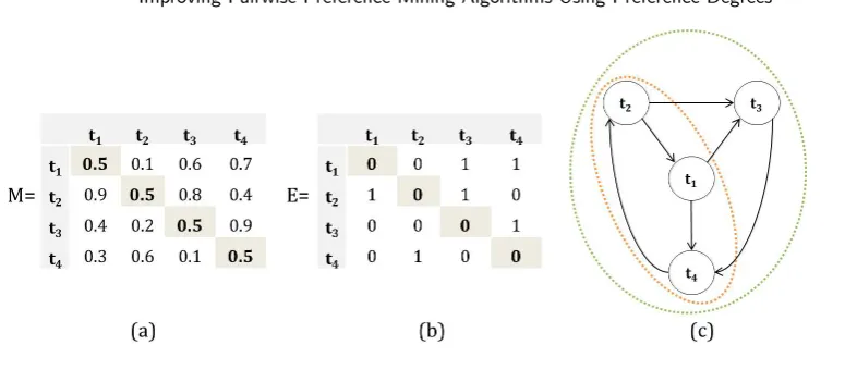
Fig. 3. (a) Fuzzy Preference RelationM, (b) Adjacency MatrixEand (c) Directed Graph.
Definition 4.1. (Adjacency Matrix): LetM be a fuzzy preference relation, an adjacency matrixE
overM is defined by:
eij =
1 ifmij≥0.5, i6=j;
0 ifmij=∗;
0 otherwise
wheremij =∗ represents an empty position in the matrix, i.e., the user has specified no preference
for this tuple pair. To illustrate, let us consider the following example:
Example 3: Let the fuzzy preference relation beM, obtained from a set of tuplesT up(R) ={t1, t2, t3, t4} illustrated in Fig. 3(a). Fig. 3(b) represents the adjacency matrix fromM obtained by Definition 4.1, while Fig. 3(c) illustrates the directed graph that represents the preferences of the matrixE. The directed edge (t1, t4) represents the fact that tuple t1 is preferred to tuplet4, which is illustrated in matrixE by the valuee14= 1.
Two size-3 cycles can be observed in the graph (Fig. 3(c)): c1(t2, t1, t4, t2) andc2(t2, t3, t4, t2), and each cycle represents a contradiction of the weak transitivity property. In order to find all these cycles, Xu et al. [2013] defines the following theorem:
Theorem 4.2. Let M be a fuzzy preference relation, E the adjacency matrix of M, and E3 the third power ofE. The number of cyclesC of a graph that represents a preference matrix is given by:
C= P
e3ij
3 , such that,i=j (1)
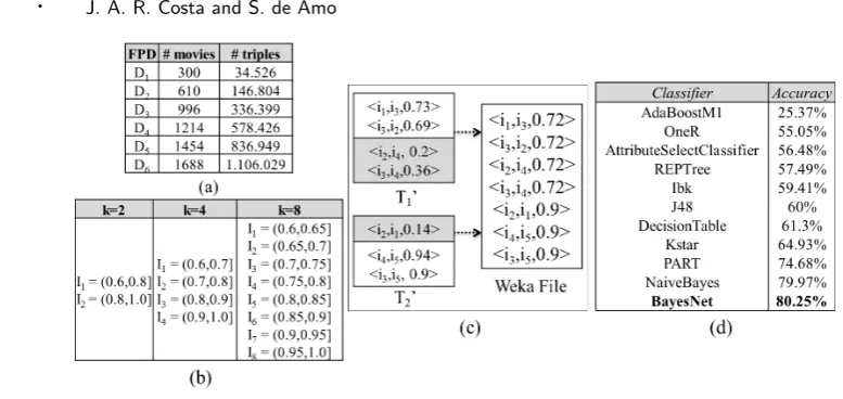
Fig. 4. (a) The FPDs, (b) The Preference Layers, (c) Preparing the training data for classification and (d) Classifier’s Accuracy.
5. EXPERIMENTAL RESULTS
5.1 Preparing the Experiments
The Fuzzy Preference Datasets (FPD).The datasets used in the experiments have been obtained
from the GroupLens Project5. The original data are of the form (UserId, FilmId, Rating). More details about the movies, namely Genre, Actors, Director, Year and Language, have been obtained by means of a crawler which extracted this information from the IMDB website6. Six datasets of film evaluations, corresponding to six different users have been considered. Details about them are shown in Fig. 4(a). For instance, dataset D1 is a set of 34.526 triples (w1, w2, n) where w1, w2 are taken from a pool of 300 movies.
Training a Classifier. A classifier is trained on each dataset in order to predict the “intensity of preference” existing between two movies. A preliminary pre-processing is needed before the classifier training phase. Each preference layer should contain 50% of triples with dp ≥ 0.5 and 50% with
dp < 0.5 in order to contain equal amount of pairs (w1, w2) with “yes” and “no” answers to “is w1 preferred tow2?”. This pre-processing is illustrated in Fig. 4(c), where the preference layers T1 and
T2 of Fig. 1(d) have been transformed into layersT10 andT20. After the calculation carried out by the fuzzification function f2 (as explained in Section 3) we havedpmin = 0.6 and dpmax = 1.0 for each
FPD considered in our experiments. The interval I = [0.6,1.0] is partitioned intoklayers, and triples of each layer receives an extra class attribute with valueλi, the averagedp for the layer. The triples
of the Weka File of Fig. 4(c) are depicted with their respective “classes”λ1= 0.72 andλ2 = 0.9. The Weka classifiers have been trained on a FPD of 31713 triples partitioned into 4 layers: T1= (0.6,0.7],
T2 = (0.7,0.8],T3= (0.8,0.9] andT4 = (0.9,1.0]. The accuracy results are shown in Fig. 4(d). The Bayesian classifiersNaive BayesandBayesNet presented the best results. Besides, they execute faster than the other ones. Thus, theBayesNet has been chosen for the remaining experiments concerning FuzzyPrefMiner evaluation.
5.2 Performance and Scalability Results
A 30-cross-validation protocol has been considered in the experiments with FuzzyPrefMiner. The FuzzyPrefMiner was implemented in Java and all the experiments were performed on a core i7 3.20GHZ
Fig. 5. Influence of Classifiers.
Fig. 6. Influence of Preference Layers.
processor, with 32GB RAM, running on operating system Linux Ubuntu 12.10. The following default values have been set for the parameters involved in the algorithm: (1)Extract Procedure: β = 50,
ϑ= 100 andγ= 20; (2) Algorithm 3: α1= 0.2 eα2= 0.2. These parameters were tested and verified in our previous work [de Amo et al. 2013]. We prefer to keep the same parameter’s values used in the CPrefMiner to make some comparisons and also the statistical significance test between these two algorithms (CPrefMiner and FuzzyPrefMiner). For evaluating theacc, prec, rec, cr, rr measures, a thresholdσ= 0.05 has been considered.
Experiments have been carried out in order to test our original claim: the more information is contained in the input data the better are the performance results. We conducted a series of experiments to validate this hypothesis and then we compare the FuzzyPrefMiner with CPrefMiner.
Influence of Classifiers. In the first test (see Fig. 4(d)), the Bayesnet classifier stands as the most performatic. However, the stratification protocol used byWeka is not the same protocol used by FuzzyPrefMiner algorithm. Therefore, we performed a second test to support us in the choice of the classifier. The main goal of this test is to analyze the influence of different classifiers when applied with FuzzyPrefMiner algorithm in crisp scenario. We chose three classifiers by analyzing the results of the first test, they are: AdaBoostM1,DecisionTable andBayesNet.
We figured out that even with a different stratification protocol theBayesNet classifier got better accuracy, recall and precision in all data sets (see Fig. 5). Regarding comparability and randomness rates, the results are quite similar in the three classifiers.
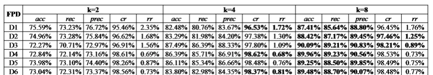
Influence of the preference layers. Intending to evaluate how the algorithm behaves according to
changes in the preference layers, we varied the number of preference layers on three levels. We divided theF P D on 2, 4 and 8 layers to analyze the performance in crisp scenario. Fig. 6 shows the results to accuracy, recall and precision. We realized that when the preference layer becomes more refined (i.e.,k= 8) better results come up.
Regarding comparability and randomness rates (see Fig. 6), we note that the results do not have significant differences. The results of allk-values are satisfactory, since we have a high comparability rate and low values of randomness rate. In this way, the FuzzyPrefMiner has good prediction because most hits are obtained by the BPN preference order.
Fig. 7. Influence ofFuzzificationFunctions.
Fig. 8. Comparison with CPrefMiner algorithm - Crisp Scenario.
Fig. 9. Comparison with CPrefMiner algorithm - Fuzzy Scenario.
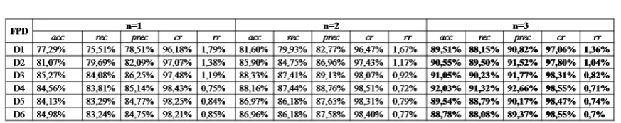
change of fuzzification function, we tested three levels of the function fn(x) = x
n
xn+1 (n= 1, n = 2
andn= 3). We consider the FuzzyPrefMiner in the fuzzy scenario and the preference layers varying according to the function. For f1, f2 and f3 we have the intervals I1 = [0.55,0.85] with 6 layers,
I2= [0.6,1.0] with 8 layers andI3= [0.65,1.0] with 7 layers, respectively. We have noticed that, the higher the value ofn(n= 3), better the results obtained for accuracy, recall and precision (see Fig. 7). For results of comparability and randomness rates, we have noticed that these results do not have significant differences. Nevertheless, for the next tests, we will fixn= 2 for thefuzzification function, because this value is an intermediate level between the functions, it has a bigger preference interval and divides the degrees of preferences better in 8 layers of the interval.
Comparison with Baseline. We consider a paired difference one tailed t-test to measure the
statistical significance of the differences between the accuracy (resp. recall, precision, comparability rate and randomness rate) of the FuzzyPrefMiner (acting in thecrisp and fuzzy scenarios) with the algorithm CPrefMiner [de Amo et al. 2013].
Both algorithms return BPNs, but CPrefMiner learns its BPN from a crisp training set and FuzzyPrefMiner from afuzzy one. We adapted the technique described in Urdan [2010] (originally designed for comparing classifiers) for our fuzzy preference mining approach. For each one of the quality measuresd0(whered0∈ {acc, rec, prec, cr, rr}) let ¯d0be the difference between thed0-measure
of the FuzzyPrefMiner (crisp and fuzzy scenarios) and the respectived0-measure the CprefMiner. The main objective of the t-test is to compute the confidence intervalγford0 and test if theNull Hypoth-esis (H0) is rejected. The confidence interval γ is calculated as follows: γ=t(1−α,k−1)×σd0, where t(1−α,k−1) is a coefficient obtained in the distribution table with (1−α) being the level of t-test and
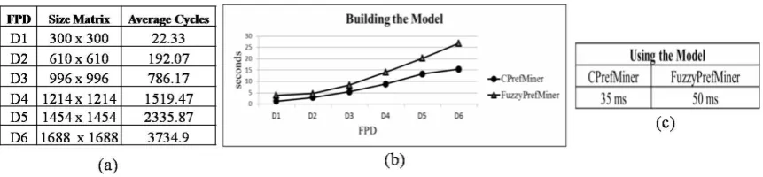
Fig. 10. (a) consistency analysis of the preference model, (b) time spent for building the models and (c) time spent for using the model on 1000 pairs of tuples.
the statistical significance for all the quality measures, because all of them were evaluated in the same size samples.
For these experiments, the main question is: With α = 0.95 of certainty, can we conclude that FuzzyPrefMiner (crisp and fuzzy scenarios) outperforms the CPrefMiner? The null and alternative hypothesis foracc,rec,precandcr areH0: FuzzyPrefMiner≤CPrefMiner andHA: FuzzyPrefMiner
>CPrefMiner. For the rr measure, the null and alternative hypothesis areH0: FuzzyPrefMiner ≥ CPrefMiner andHA: FuzzyPrefMiner<CPrefMiner. The Fig. 8 and Fig. 9 show the results and the statistical significance test to compare the FuzzyPrefMiner with CPrefMiner. The results (crisp and fuzzy scenarios) show that for accuracy, recall and precision measures theH0 is rejected (since all the values contained in the confidence interval are positive), and, for these measuresHAis substantiated. As for the comparability and randomness rate measures, theH0 is rejected in some FPD such asD4 andD5, and thus,HAis substantiated for these cases and for others FPD (D1,D2,D3 andD6) the observed differences has not statistical significance.
These results show the superiority of FuzzyPrefMiner over CPrefMiner, even when validated in the fuzzy scenario. As expected the performance of FuzzyPrefMiner in thefuzzy scenario decreases with respect to its performance in thecrisp scenario, since the fuzzy validation protocol requires predicting the degree of preference between two tuples and not only their relative preference ordering.
Execution Time. Fig. 10(b) presents the time spent by CPrefMiner and FuzzyPrefMiner to build
their respective models. In the case of FuzzyPrefMiner the total time includes the time spent for pre-processing the input data for the classifier (involving I/O operations), the time spent by the classifier BayesNet to build the classification model and the time spent to mine the 8 BPNs, one for each partition. As expected, FuzzyPrefMiner is more costly than CPrefMiner.
The Fig. 10(c) shows the time spent to predict the preference for 1000 pairs of tuples. Again, FuzzyPrefMiner is a little more costly than CPrefMiner taking nearly 1.4T3, where T3 is the time spent by CPrefMiner to accomplish the same task.
Consistency Analysis. We analyzed the consistency of preference model, based on the amount
6. CONCLUSION
We studied the influence of thedegree of preferencein the performance of Preference Mining techniques specific for learning contextual preference models and propose the algorithm FuzzyPrefMiner for this task, with very promising results. We have fixed the parameter σ = 0.05 to the experiments in this paper. However, it is intended to change this value in futures works, as well as apply others fuzzification functions found in the literature.
Other future research concentrates on the design of techniques for repairing inconsistency in the fuzzy relation produced by FuzzyPrefMiner. Although the original BPN introduced in our previous works is capable to infer a strict partial order on the set of tuples, the fuzzy relation produced by FuzzyPrefMiner does not verify some transitivity properties of fuzzy relations such as weak transitivity or additive transitivity [Herrera-Viedma et al. 2004].
REFERENCES
Burges, C. J. C.,Shaked, T.,Renshaw, E.,Lazier, A.,Deeds, M.,Hamilton, N.,and Hullender, G. N.Learning to Rank Using Gradient Descent. InProceedings of the International Conference on Machine Learning. New York, NY, USA, pp. 89–96, 2005.
Chiclana, F.,Herrera, F.,and Herrera-Viedma, E.Integrating three representation models in fuzzy multipurpose decision-making based on fuzzy preference relations.Fuzzy Sets and Systems 97 (1): 33–48, 1998.
Cohen, W. W.,Schapire, R. E., and Singer, Y. Learning to Order Things. Journal of Artificial Intelligence Research10 (1): 243–270, 1999.
Crammer, K. and Singer, Y. Pranking with Ranking. InProceedings of the International Conference on Neural Information Processing Systems: Natural and Synthetic. Vancouver, Canada, pp. 641–647, 2001.
de Amo, S.,Bueno, M. L. P.,Alves, G.,and da Silva, N. F. F. Mining User Contextual Preferences. Journal of Information and Data Management4 (1): 37–46, 2013.
de Amo, S.,Diallo, M. S.,Diop, C. T.,Giacometti, A.,Li, H. D.,and Soulet, A. Mining Contextual Preference Rules for Building User Profiles. InProceedings of International Conference on Data Warehousing and Knowledge Discovery. Vienna, Austria, pp. 229–242, 2012.
Freund, Y.,Iyer, R.,Schapire, R. E.,and Singer, Y.An Efficient Boosting Algorithm for Combining Preferences.
The Journal of Machine Learning Researchvol. 4, pp. 933–969, 2003.
Herrera-Viedma, E.,Herrera, F.,Chiclana, F.,and Luque, M. Some Issues on Consistency of Fuzzy Preference Relations.European Journal of Operational Research154 (1): 98–109, 2004.
Jiang, B.,Pei, J.,Lin, X.,Cheung, D. W.,and Han, J.Mining Preferences from Superior and Inferior Examples. In
Proceedings of the ACM SIGKDD International Conference on Knowledge Discovery and Data Mining. Las Vegas, USA, pp. 390–398, 2008.
Joachims, T.Optimizing Search Engines Using Clickthrough Data. InProceedings of the ACM SIGKDD International
Conference on Knowledge Discovery and Data Mining. Edmonton, Canada, pp. 133–142, 2002.
Koriche, F. and Zanuttini, B.Learning Conditional Preference Networks. Artificial Intelligence174 (11): 685–703, 2010.
Ma, J.,Fan, Z.-P., Jiang, Y.-P., Mao, J.-Y., and Ma, L. A Method for Repairing the Inconsistency of Fuzzy Preference Relations.Fuzzy Sets and Systems 157 (1): 20–33, 2006.
Urdan, T. C.Statistics in Plain English. Taylor & Francis, 2010.
Wilson, N. Extending CP-Nets with Stronger Conditional Preference Statements. In Proceedings of the National Conference on Artificial Intelligence. San Jose, CA, USA, pp. 735–741, 2004.
Xu, Y.,Patnayakuni, R.,and Wang, H. The Ordinal Consistency of a Fuzzy Preference Relation. Information