R E S E A R C H A R T I C L E
Open Access
Performance of Firth-and
log
F
-type
penalized methods in risk prediction for small
or sparse binary data
M. Shafiqur Rahman
*and Mahbuba Sultana
Abstract
Background: When developing risk models for binary data with small or sparse data sets, the standard maximum likelihood estimation (MLE) based logistic regression faces several problems including biased or infinite estimate of the regression coefficient and frequent convergence failure of the likelihood due to separation. The problem of separation occurs commonly even if sample size is large but there is sufficient number of strong predictors. In the presence of separation, even if one develops the model, it produces overfitted model with poor predictive
performance. Firth-and logF-type penalized regression methods are popular alternative to MLE, particularly for solving separation-problem. Despite the attractive advantages, their use in risk prediction is very limited. This paper evaluated these methods in risk prediction in comparison with MLE and other commonly used penalized methods such as ridge.
Methods: The predictive performance of the methods was evaluated through assessing calibration, discrimination and overall predictive performance using an extensive simulation study. Further an illustration of the methods were provided using a real data example with low prevalence of outcome.
Results: The MLE showed poor performance in risk prediction in small or sparse data sets. All penalized methods offered some improvements in calibration, discrimination and overall predictive performance. Although the Firth-and logF-type methods showed almost equal amount of improvement, Firth-type penalization produces some bias in the average predicted probability, and the amount of bias is even larger than that produced by MLE. Of the logF(1, 1)and logF(2, 2)penalization, logF(2, 2)provides slight bias in the estimate of regression coefficient of binary predictor and logF(1, 1)performed better in all aspects. Similarly, ridge performed well in discrimination and overall predictive performance but it often produces underfitted model and has high rate of convergence failure (even the rate is higher than that for MLE), probably due to the separation problem.
Conclusions: The logF-type penalized method, particularly logF(1, 1)could be used in practice when developing risk model for small or sparse data sets.
Keywords: Prediction model, Separation, Performance measures, Overfitting
Background
In many areas of clinical research, risk models for binary data are usually developed in the maximum-likelihood (ML) based logistic regression framework to predict the risk of a patient’s future health status such as death or illness [1, 2]. For example, in cardiology, models may be developed to predict the risk of having cardiovascu-lar disease. Predictions based on these models are useful
*Correspondence: [email protected]
Institute of Statistical Research and Training, University of Dhaka, Dhaka, Bangladesh
to both doctor and patient in making joint decision on future course of treatment. However, before using these models in risk prediction it is essential to assess their pre-dictive performance using data other than that used to develop the models, which is termed as ‘validation’ [3, 4]. A good risk model is expected to demonstrate good cal-ibration (accuracy of prediction) and discrimination (the ability of model to distinguish between low-and-high risk patients) in new dataset. A risk model that perform well in development data (that used to fit the model called ‘training’ set) may not perform similar to the validation
data (that used to validate the model called ‘test’ set). One of the main reasons for not performing well in test data is model overfitting which causes too high prediction for high risk patients and too low for low risk patients. The overfitting occurs frequently when the number of events in training data is lower than the number of risk factors. After employing expert knowledge even if one fits the model with reduced the number of predictors, the ratio of the number of event to the number of predictors (EPV) often very low. However, as a rule of thumb, it has been suggested in literature that the risk model performs well when EPV is at least 10 [5]. Although the choice of this cut-off has some criticisms [6] for not being based on sci-entific reasoning except empirical evidence, it is found useful for quantifying the amount of information in the data relative to model complexity [7, 8]. However, the requirement of minimum EPV is often difficult to achieve when the risk models develop for low-dimensional data with rare outcome or small-and moderate-size, and for high-dimensional data where the number of pre-dictors is usually higher than the number of sample observations.
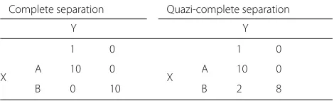
To overcome the problem related to overfitting, some studies [9, 10] explored the use of penalized regression methods in risk prediction. Of them Ambler et al. [9] explored the use of two popular penalized regression methods, such as ridge [11] and lasso [12], in risk pre-diction for low-dimensional survival data with rare events and found that both methods improve calibration and discrimination compared with the ML based standard Cox models. Pavlou et al. [10] reviewed and evaluated ridge and lasso and their some extensions, such as elas-tic net, adaptive lasso etc [13–15], in risk prediction for low dimensional binary data with rare events and found that these methods can offers improvement, particularly for model overfitting, over the standard logistic regression model. Although these studies showed some improve-ment in risk prediction for rare-event data by using the penalized methods, there is no specific guidelines how risk prediction can be managed in the presence of separa-tion, which frequently occur for such rare-event or sparse data. More specifically, the problem of separation, first reported by Albert and Anderson [16], is the case where one or more predictors have strong effects on response and hence (nearly ) perfectly predict the outcome of inter-est. Table 1 presents an example of both complete (perfect prediction) and quazi-complete separation (nearly perfect prediction) caused by a dichotomous predictorXagainst binary outcomeY.
Separation may occur even if the data is large but there is sufficient number of strong predictors. The likelihood of separation is higher for categorical predictors with rare category compared to the continuous predictor [17]. When developing model in the presence of separation, ML
Table 1Example of separation due to a dichotomous predictor
Xagainst outcomeY
Complete separation Quazi-complete separation
Y Y
1 0 1 0
X A 10 0 X A 10 0
B 0 10 B 2 8
Number in each cell indicates number of observations
based logistic regression faces several problems [16, 18]. These includes lack of convergence of maximum likeli-hood and even if it converges it produces biased (some-times infinite) estimate of the regression coefficient [17]. An alternative to the ML approach in this situation is Firth’s penalized method [19]. This approach removes the first order term (O(n−1)) in the asymptotic bias expansion of the MLEs of the regression parameters by modifying the score equation with a penalty terms known as Jef-freys invariant prior. Heinze and Schemper [17] provided an application of Firth’s method to the solution of the problem of separation in the logistic regression. Further the applications of Firth’s method have been provided to proportional and conditional logistic regressions for sit-uations with small-sample bias reduction and solution to problem of separation [20, 21].
However, one of the criticisms of Firth-type penalty in recent studies [22, 23] is that it depends on observed covariate data which can lead to artifacts such as esti-mates lying outside the range of prior median and the MLE (which is known as Bayesian non-collapsibility). An alternative to this, Greenland and Mansournia [22, 23] suggested logF(1, 1)and logF(2, 2)priors as default prior for logistic regression. As argued by the authors, the proposed logF priors are transparent, computationally simple, and reasonable for logistic regression. However, despite the attractive advantages of these penalized meth-ods including Firth’s method for sparse or small data sets, limited studies have been conducted to explore their use in risk prediction. This paper evaluates the predictive per-formance of these penalized methods for sparse data and compares the results with the ML based method and the other commonly used penalized method such as ridge. Although lasso is a commonly used method, it is popular for variable selection. Risk prediction and variable selec-tion are different issues, and in this paper we have focused on prediction and hence excluded lasso.
Methods
Maximum likelihood based logistic regression model LetYi,(i= 1, 2,. . .,n), be a binary outcome (0/1) for the
ith subject which follows Bernoulli distribution with the probabilityπi=Pr(Yi=1). The logistic regression model
can be defined as
logit[πi|xi)]=ηi=βTxi,
whereβT is a vector of regression coefficients of length (k+1), andxiis theith row vector of the predictor matrix
xwhich has ordern×(k+1). The termηi=βTxiis called
as risk score or ‘prognostic index’.
In standard MLE, the model is fitted by maximizing the log likelihood denoted byl(β).
Penalized methods for logistic regression model
Whereas in penalized methods, l(β) is maximized sub-ject to constraints on the values of regression coefficients. The constraints are fixed in such a way so that the regres-sion coefficient shrinks towards zero in comparison with MLE, which may help to alleviate overfitting. More specif-ically, the penalized regression coefficient is obtained by maximizing the penalized log likelihood denoted by ł(β)− pen(β), where pen(β) is the ‘penalty term’. The penalty term is the functional form of constraints. The penal-ized methods differ from each others in the choice of penalty term. The following subsection briefly discusses some popular penalized methods.
Firth’s penalized method
In order to remove first order bias in MLEs of the regres-sion coefficient, Firth [19] suggested to use penalty term
1
2trace[I(β)−1∂I(β)/∂βj] in the ML based score equation U(βj)=∂l(β)/∂βj=0. The modified score equations are
thenU(βj)∗ = U(βj) +1/2trace[I(β)−1∂I(β)/∂βj]= 0
(j = 1,. . .,k), where I(β)−1 is the inverse of informa-tion matrix evaluated atβ. The corresponding penalized log-likelihood function for the above modified score func-tion isl(β)+1/2 log|I(β)|. The penalty term used above is known as Jeffreys invariant prior and its influence is asymptotically negligible. The Firth type penalized MLE of β is thus βˆ = argmaxl(β)+1/2 log|I(β)|. This approach is known as bias preventive rather than cor-rective. However, Greenland and Mansournia [23] identi-fied some problems in Jeffreys prior (equivalent to Firth’s penalty term). These includes i)Jeffrey’s prior is data-dependent and includes correlation between covariates ii) the marginal prior for a givenβcan change in opaque ways as model covariates are added or deleted, which may pro-vide surprising results in sparse dataset, and iii) it is not clear how the penalty translate into prior probabilities for odds ratios.
Penalized method based onlogFprior
To overcome these problems, Greenland and Mansournia [23] proposed a class of penalty functions pen(β) = ln(|I(β)|−m)indexed bym ≥ 0, which produce MLE for m = 0. Then the penalized log-likelihood is equal to l(β)+mβ/2−mln(1+eβ). They showed that the antilog of the penalty termmβ/2−mln(1+eβ)is proportional to a logF(m,m)density forβ, which is the conjugate fam-ily for binomial logistic regression [24, 25]. It is noted that the prior degrees of freedomm in logF prior is exactly the number of observations added by the prior. Then the corresponding penalized ML estimate can be obtained as
ˆ
β = argmaxl(β)+mβ/2−mln(1+eβ). This shows that βˆ has first order (O(n−1)) bias of zero form = 1, away from zero form < 1, and shrinks toward zero for m>1. This showed thatF(0, 0)is equivalent to MLE, and F(1, 1) includes Jefrreys prior in one parameter model, for example, matched pair case-control. Greenland and Mansournia strongly argued against imposing a prior on the intercept to make sure that the mean predicted prob-ability of binary condition is equal to the proportion of events. In this study, we focused on F(1, 1) andF(2, 2) prior for computational simplicity.
Ridge penalized method
Le Cessie and van Houwelingen [11] uses the penalty term asλ2kj=1βj2, whereλ2is a tuning parameter that
mod-ulates the trade-off between the likelihood term and the penalty term and is usually selected as data-driven pro-cedure such as cross validation. The ridge log-likelihood is thus defined as l(β) − λ2jk=1βj2 and hence βˆ =
argmax
l(β)−λ2kj=1βj2
. Ridge was initially devel-oped to solve the problems due to multicolinearity. How-ever, it shrinks the regression coefficient towards nearly zero and hence can be performed well to alleviate over-fitting in risk prediction in the scenario with correlated predictors.
Evaluating predictive performance
Three common approaches to evaluate the predictive per-formance of a risk model [26]. These are i) calibration (the agreement between the observed and predicted risk in a group of subjects) ii) discrimination (the ability of model to distinguish between low-and high-risk patients) iii) overall prediction accuracy.
Calibration: We assessed calibration by calculating cali-bration slope, which can be obtained by re-fitting a binary logistic regression model with linear predictor or prog-nostic index (PI) derived from the original model as the only predictor. The estimated slopeβˆPI is the calibration
slope. IfβˆPI = 1, it suggests perfect calibration;βˆPI < 1
Discrimination: We assessed discriminating ability of the model by quantifying the area under receiver oper-ating characteristic curve (AUC), graph of sensitivity positive rate) versus one minus specificity (true-negative rate) evaluated at consecutive threshold val-ues of the predicted risk score or probability derived from the model. Alternatively AUC can be obtained by quantifying the probability that, for a randomly selected pair of subjects, the subject who experienced the event of interest had higher predicted risk derived from the model than those without experiencing the event. A value AUC=0.5 indicates no discrimination and 1 suggest perfect discrimination.
Overall predictive performance: The overall prediction accuracy is quantified using Brier score, which is the mean of the squared difference between the observed and pre-dicted risk for each patient derived from the model. The lower the BS, the better the prediction of a model and BS=0 indicates perfect prediction. For ease of interpre-tation we reported root BS(rBS). In addition to the rBS, we also reported average predictive probability (APP) of the model to see how the predicted value differ from the corresponding observed value.
Software
All the analyses and simulations were conducted in Stata version 12. Several Stata packages and functions were used to fit the models in different methods under study. These includes ‘logit’, ‘firthlogit’, ‘penlogit’, and ‘plogit’ along with ‘plsearch’ for MLE, FIRTH, logF and RIDGE, respectively. The calculation of calibration slope and Brier score were performed using self written Stata code and AUC using the package ‘roctab’.
Results
Example data: stress echocardiography data
The dataset used for simulation and illustration is in public domain and originally extracted from the study conducted by Krivokapich et al. [27] where the aim was to quantify the prognostic value of dobutamine stress echocardiography (DSE) in predicting cardiac events in 558 patients (male 220 and female 338) with known or suspected coronary artery disease. The responses of inter-est whether or not a patient suffered from either of ‘death due to cardiac arrest’, or ‘ myocardial infarction (MI)’, or ‘ revascularization by percutaneous transluminal coronary angioplasty (PTCA)’ or ‘coronary artery bypass grafting surgery (CABG)’ over the next year after having the test. There were 24 patients with cardiac death, 28 with MI, 27 with PTCA, 33 with CABG and 89 with any cardiac event (Cevent), which implies that the each of the events was rare. The main predictor of interest are age, history of hypertension (HT: yes/no) and diabetics mellitus (DM:
yes/no), history of prior MI (yes/no) and PTCA (yes/no), status of DSE test (positive DSE:positive/negative), wall motion anamoly on echocardiogram (rest WMA:yes/no), ejection fraction on dobutamine(Dobutamine EF), and base ejection fraction (base EF).
Simulation study
The performance of the penalized methods in risk pre-diction over standard ML based logistic regression were investigated using a simulation study. We conducted sim-ulation i) firstly to assess and compare the properties of the regression coefficients of the different methods (MLE, FIRTH, logF(1, 1), logF(2, 2), RIDGE) under study and ii) secondly to assess and compare the predictive perfor-mance between the methods.
Assessing the properties of the regression coefficients
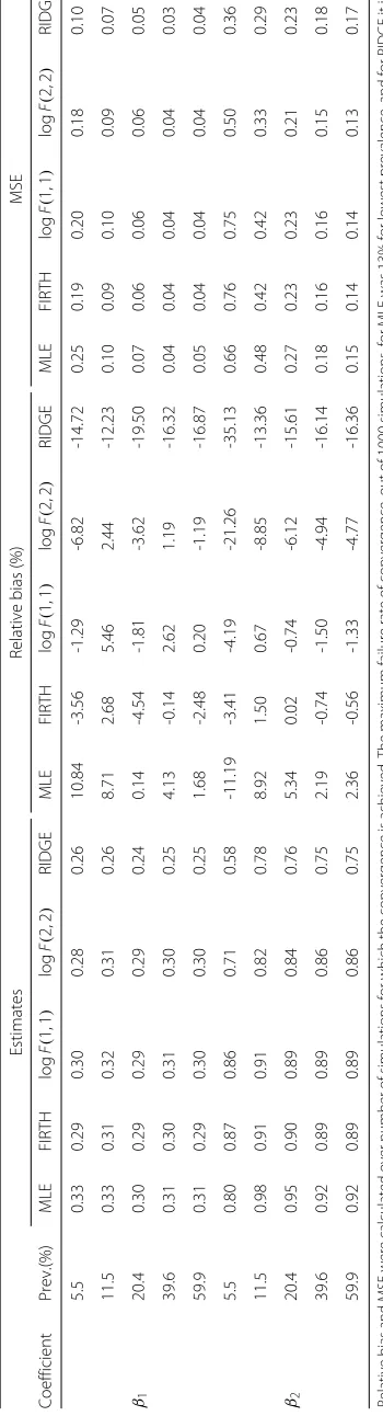
To assess the properties of the regression coefficients such as bias and mean squared error (MSE), we generated two independent predictors of which one is continuous (X1) generated from standard normal and the other is dichoto-mous (X2) generated from Bernoulli distribution with 50% events. We then generated binary response from Bernoulli distribution with probabilityπi (i = 1,. . .,n) calculated
from true logistic model logit(π) = β0+β1X1+β2X2, where β1 = 0.30 and β2 = 0.9. With this combina-tion, the binary covariate created separation for some of the simulated datasets particularly with low preva-lence. The value ofβ0vary to generate data with varying level of prevalence. The scenarios were created by vary-ing the prevalence, on an average, (p) as 5.5, 11.5 20.4 and 39.6% for a fixed sample size n = 120. For each scenario, 1000 datasets were generated and all regression approaches under study were fitted to each dataset. When fitting RIDGE the respective tuning parameters were selected through 10-fold cross validation. The estimates of the regression coefficients of the respective models were obtained as the mean over the number of simulations where convergence achieved. Noted that only MLE and RIDGE were failed to converge (due to low prevalence or separation or both) in some datasets, and the maxi-mum failure rate for MLE and RIDGE were 13 and 51% , respectively for the lowest prevalence scenario. The fail-ure rate decreases as the prevalence increases. Finally the relative bias (%) and mean squared error (MSE) of the esti-mates were reported and compared if the performance vary across the scenarios.
for the low prevalence data and the lowest for the high prevalence data. However, the RIDGE, in general, pro-duces the lowest MSE, and the highest MSE is produced by the MLE forβ1and by FIRTH forβ2. The amount of MSE, in general, decreases with the increasing prevalence.
Assessing the predictive performance
To assess the predictive performance of the methods, we conducted two simulation series following the simula-tion design in Pavlou et al. [10] used for similar type of study. The first simulation series is based on the real stress echocardiography data where only responses were gen-erated and in the second simulation series we gengen-erated both covariates and responses.
Stress echocardiography simulation
In the first simulation series based on real data, we sim-ulated data and evaluated the predictive performance of the models for different EPV scenarios using the following steps:
(i) Fit the following logistic regression model for the response “any cardiac event” with Firth’s penalized method (to avoid bias in the estimate of the regression coefficient) to obtain the true model:
logit(Pr(Cevent=1))=β0+β1dobef+β2wma+β3posse
+β4bsef +β5ht+β6age
(ii) To create a training data, choose the EPV and prevalence (prev), and then calculate sample size for the respective EPV given the number of predictorsp asn= EPVprev×p. Sample with replacement then values of the covariates in the true model from original data. For each of then values of the covariates, simulate new responses from Bernoulli distribution with the probability calculated from the fitted model. However, replace the value ofβ0by -0.65 to confirm the prevalence of the response (prev), on an average, 15.5% for all EPV scenarios.
(iii) With this combination, check and record if separation occurred due to any of the binary covariates (‘posse’ or ‘wma’, or ‘ht’ or combination of them). Otherwise to create separation, enlarge the true value of the respective coefficient of the binary covariate to some extents. Note that the chances of separation is expected to increase with decreasing EPV value. (iv) To create a test dataset, sample with replacement
m×n(m times of the original data of sizen=558, we consideredm=2) values of the covariates. Then simulate the corresponding new responses from the same true model used for simulating training data. (v) Repeat the steps (ii)-(iii) to produce 1000 training and
1000 test datasets.
(vi) Fit the risk models ( using MLE and all types of
penalized regression methods under study) to each of the training data sets and check whether convergence was achieved. Then evaluate their predictive
performance (if convergence achieved) by means of calibration slope, AUC, root Brier score, and average predictive probability (APP) using the corresponding test dataset. Summarize the predictive performance over the number of simulations for which
convergence is achieved.
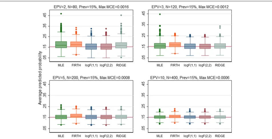
The predictive performance of all regression methods was investigated against EPV=2, 3, 5, 10 to see if the performance vary across the scenarios. When the pre-dictive performance against EPV was assessed by means of calibration slope, the MLE showed poor performance by producing overfitted model (calibration slope substan-tially lower than 1) for EPV=2, 3, 5 (Fig. 1). All penalized methods offered improvement to some extents except the RIDGE which produced underfitted model ( the average value of the calibration slope greater than 1 with high SD). In addition, the RIDGE failed to converge for the maxi-mum 8.4% of the simulations particularly when EPV=2. Almost equal improvement was offered by the Firth-type and both the logF(1, 1) and logF(2, 2) penalized meth-ods. In general all methods including MLE showed almost equal performance in terms of calibration for high EPV (EPV=10). When the predictive performance (discrimi-natory ability) was assessed through AUC, all penalized methods showed better performance with greater AUC than MLE for the low EPV scenarios (Fig. 2). Of them the RIDGE provided highest AUC value. However, the amount of improvement in the discrimination, in gen-eral, was comparatively lower than that for calibration. All methods perform almost equally for high EPV (EPV=10). Similarly the penalized methods offered improvement in the overall predictive performance for individual predic-tion assessed through rBS to some extents for low EPV (Fig. 3). Of them, the RIDGE offered greater improve-ment. However, for low EPV while both the logF(1, 1)and logF(2, 2)penalized methods provided accurate estimate of the true average predicted probability (APP) 15.2%, the FIRTH-type penalized method overestimate the true value. The amount of bias in FIRTH-type estimate is even larger than that produced by MLE and RIDGE (Fig. 4).
Further simulation
In the second simulation series with the same EPV scenar-ios, we simulated both covariates and response under two predictive models, one with weak predictive ability and the other with strong predictive ability, using the following steps:
Fig. 1Performance of the methods was assessed using calibration slope and compared. Results were summarized over the number of simulations for which convergence is achieved. The maximum failure rate of convergence for RIDGE, out of 1000 simulations, is 8.4% when EPV=2. The values outside the whisker were not plotted to make the plot readable. Thehorizontal dash lineis the median calibration slope for MLE and thesolide lineis the optimal value
the given EPV value and the number of predictors using the same formula previously used.
(ii) For each observation in training data, first simulate three continuous predictors (X1,X2,X3)
independently from standard normal distribution and
two binary predictors (X4,X5) independently from Bernoulli distribution one with low (20%) and the other with high (60%) prevalence.
(iii) Simulate the corresponding responses from Bernoulli dis-tribution with probability calculated from the true model:
Fig. 2Performance of the methods was assessed using area under ROC (AUC) and compared. Results were summarized over the number of
simulations for which convergence is achieved. The maximum failure rate of convergence for RIDGE, out of 1000 simulations, is 8.4% when EPV=2.
Fig. 3Performance of the methods was assessed using root Brier score (rBS) and compared. Results were summarized over the number of simulations for which convergence is achieved. The maximum failure rate of convergence for RIDGE, out of 1000 simulations, is 8.4% when EPV=2.
Thehorizontal solide lineis the median rBS for MLE
logit(π)=β0+β1X1+β2X2+β3X3+β4X4+β5X5.
For the model with weak predictive ability, the values of the regression coefficient were set asβ0= −1.5β1= 0.2,β2=0.5β3= −0.03,β4=0.05andβ5= −0.6
and for the model with strong predictive ability, the corresponding true values were set asβ0= −3.5, β1=1.2,β2= −0.9β3=0.9,β4=1.2andβ5=1.2. In each case, the value of theβ0confirms the desired prevalence of the response. With this combination,
Fig. 4Performance of the methods was assessed using Average Predicted Probability (APP) and compared. Results were summarized over the
the binary covaritesX5in the model with weak predictive ability andX4in the model with strong predictive ability create separation in some of the simulations. Check and record if separation occurred. (iv) Create test data with size 1000 (much larger than the
training data) for the similar level of EPV and prevalence. For each observation in the test data, simulate the same predictors as in the test data and the corresponding response from the same true model.
(v) Repeat the steps (ii)-(iv) to produce 1000 training and 1000 test datasets
(vi) Fit risk models (using all methods) using training data, count if convergence was achieved for the respective model, and evaluate their predictive performance (if convergence was achieved in training data) using test data as before. Finally summarize the predictive performance over the number of
simulations for which convergence is achieved.
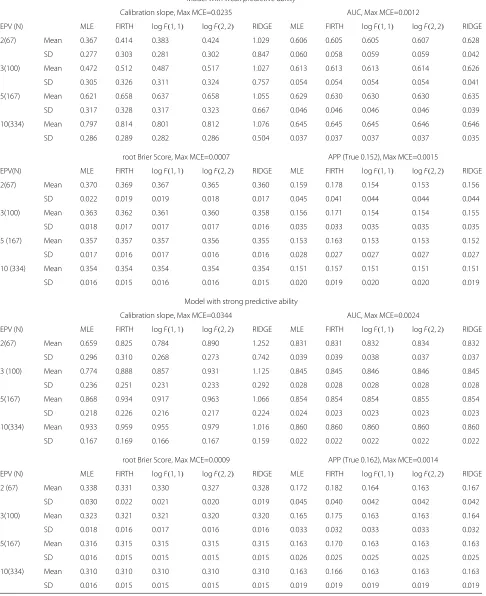
The results revealed that, for both predictive models (weak and strong predictive abilities), all the penalized methods offered improvement in calibration over MLE for low EPV, except for the RIDGE which in turn pro-vided underfitted model (calibration slope grater than 1 with high SD) (Table 3). The amount of improvement by the other penalized methods was almost equal. However, all the penalized methods except the RIDGE offered neg-ligible improvement in the discrimination for low EPV. Similarly all the penalized methods showed improvement to some extents in the overall predictive performance by lowering the rBS value compared to that for MLE. For both predictive model, the average predicted probability (APP) estimated by the both the logF(1, 1)and logF(2, 2) were almost equal to the average observed probability, however the Firth-type penalized method introduced pos-itive bias in the estimate of the average probability. The amount of bias was even larger than that for MLE and RIDGE. In case of both models, the maximum failure of convergence (due to separation or low EPV or both) was reported for RIDGE.
Illustration using stress echocardiography data
The aim is to derive risk models using different penal-ized methods discussed earlier and the standard MLE to predict the risk of having a cardiac event and then to eval-uate and compare their predictive performance. We fitted separate models for predicting the risk of each of the four cardiac events and a model for the risk of any of the events using each regression approaches; that is, a total of five models for each of the binary events were fitted using six different regression methods under study and altogether 25 models for all five binary responses.
The models were fitted using training data (contains
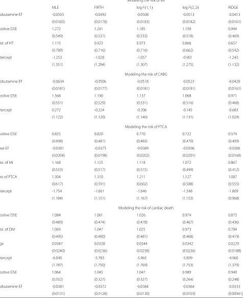
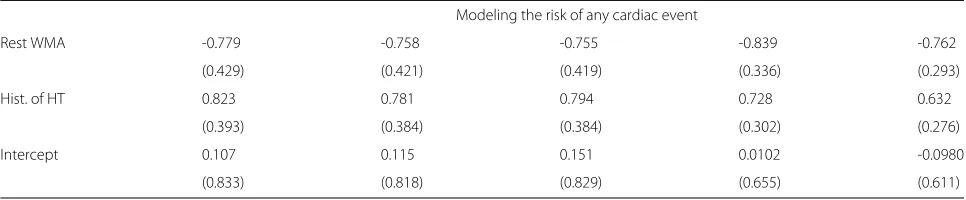
60% of total data randomly selected) and their predic-tive performance were evaluated using test data (contains rest of 40%). The associated predictors for each car-diac event were selected based on the information from literature and results of likelihood ratio test (LRT). Dif-ferent combinations of predictors were tested using LRT to come up with a final model for each cardiac event. Then the same model was then fitted in training data using six different methods. Note that quasi-complete separation due to binary predictors in training data was identified for the responses ‘PTCA’ and ‘ cardiac death’, and hence, in case of convergence failure for RIDGE or MLE, the estimates reported are based on the last iteration. The estimated coefficients of the respective model are then summarized in Table 4. For all types of response, the estimated regression coefficients for MLE is larger than all penalized methods. Because all the meth-ods shrink the coefficient towards zero. The amount of shrinking was higher for the RIDGE in the most of the cases. However, the main purpose here is to evaluate the predictive performance of the methods rather than comparing their estimated regression coefficients. The predictive performance of all models were then evalu-ated using test data, and the results were summarized in Table 5.
It is observed from results in Table 5 that all models faced the problem of overfitting (calibration slope << 1) particularly for those response for which the EPV is low (EPV<10). The amount of overfitting is lower for all penalized methods compared to MLE. In terms of discrimination all methods including MLE provided com-parable results. For all types of response, the greater improvement was observed in the calibration (calibration slope) compared to those in both discrimination (AUC) and overall performance (BS). Firth methods produced higher value of the average predicted probability (APP) for all type of responses.
Table 3Performance measures for the model s with both weak and strong predictive ability. Results were summarized over the number of simulations for which convergence is achieved. The maximum failure rate of convergence for RIDGE with weak predictive ability, out of 1000 simulations, is 40% for the lowest EPV
Model with weak predictive ability
Calibration slope, Max MCE=0.0235 AUC, Max MCE=0.0012
EPV (N) MLE FIRTH logF(1, 1) logF(2, 2) RIDGE MLE FIRTH logF(1, 1) logF(2, 2) RIDGE
2(67) Mean 0.367 0.414 0.383 0.424 1.029 0.606 0.605 0.605 0.607 0.628
SD 0.277 0.303 0.281 0.302 0.847 0.060 0.058 0.059 0.059 0.042
3(100) Mean 0.472 0.512 0.487 0.517 1.027 0.613 0.613 0.613 0.614 0.626
SD 0.305 0.326 0.311 0.324 0.757 0.054 0.054 0.054 0.054 0.041
5(167) Mean 0.621 0.658 0.637 0.658 1.055 0.629 0.630 0.630 0.630 0.635
SD 0.317 0.328 0.317 0.323 0.667 0.046 0.046 0.046 0.046 0.039
10(334) Mean 0.797 0.814 0.801 0.812 1.076 0.645 0.645 0.645 0.646 0.646
SD 0.286 0.289 0.282 0.286 0.504 0.037 0.037 0.037 0.037 0.035
root Brier Score, Max MCE=0.0007 APP (True 0.152), Max MCE=0.0015
EPV(N) MLE FIRTH logF(1, 1) logF(2, 2) RIDGE MLE FIRTH logF(1, 1) logF(2, 2) RIDGE
2(67) Mean 0.370 0.369 0.367 0.365 0.360 0.159 0.178 0.154 0.153 0.156
SD 0.022 0.019 0.019 0.018 0.017 0.045 0.041 0.044 0.044 0.044
3(100) Mean 0.363 0.362 0.361 0.360 0.358 0.156 0.171 0.154 0.154 0.155
SD 0.018 0.017 0.017 0.017 0.016 0.035 0.033 0.035 0.035 0.035
5 (167) Mean 0.357 0.357 0.357 0.356 0.355 0.153 0.163 0.153 0.153 0.152
SD 0.017 0.016 0.017 0.016 0.016 0.028 0.027 0.027 0.027 0.027
10 (334) Mean 0.354 0.354 0.354 0.354 0.354 0.151 0.157 0.151 0.151 0.151
SD 0.016 0.015 0.016 0.016 0.015 0.020 0.019 0.020 0.020 0.019
Model with strong predictive ability
Calibration slope, Max MCE=0.0344 AUC, Max MCE=0.0024
EPV (N) MLE FIRTH logF(1, 1) logF(2, 2) RIDGE MLE FIRTH logF(1, 1) logF(2, 2) RIDGE
2(67) Mean 0.659 0.825 0.784 0.890 1.252 0.831 0.831 0.832 0.834 0.832
SD 0.296 0.310 0.268 0.273 0.742 0.039 0.039 0.038 0.037 0.037
3 (100) Mean 0.774 0.888 0.857 0.931 1.125 0.845 0.845 0.846 0.846 0.845
SD 0.236 0.251 0.231 0.233 0.292 0.028 0.028 0.028 0.028 0.028
5(167) Mean 0.868 0.934 0.917 0.963 1.066 0.854 0.854 0.854 0.855 0.854
SD 0.218 0.226 0.216 0.217 0.224 0.024 0.023 0.023 0.023 0.023
10(334) Mean 0.933 0.959 0.955 0.979 1.016 0.860 0.860 0.860 0.860 0.860
SD 0.167 0.169 0.166 0.167 0.159 0.022 0.022 0.022 0.022 0.022
root Brier Score, Max MCE=0.0009 APP (True 0.162), Max MCE=0.0014
EPV (N) MLE FIRTH logF(1, 1) logF(2, 2) RIDGE MLE FIRTH logF(1, 1) logF(2, 2) RIDGE
2 (67) Mean 0.338 0.331 0.330 0.327 0.328 0.172 0.182 0.164 0.163 0.167
SD 0.030 0.022 0.021 0.020 0.019 0.045 0.040 0.042 0.042 0.042
3(100) Mean 0.323 0.321 0.321 0.320 0.320 0.165 0.175 0.163 0.163 0.164
SD 0.018 0.016 0.017 0.016 0.016 0.033 0.032 0.033 0.033 0.032
5(167) Mean 0.316 0.315 0.315 0.315 0.315 0.163 0.170 0.163 0.163 0.163
SD 0.016 0.015 0.015 0.015 0.015 0.026 0.025 0.025 0.025 0.025
10(334) Mean 0.310 0.310 0.310 0.310 0.310 0.163 0.166 0.163 0.163 0.163
SD 0.016 0.015 0.015 0.015 0.015 0.019 0.019 0.019 0.019 0.019
Table 4Modeling the risk of cardiac events. Estimate of the regression coefficients with SE in the parenthesis
Modeling the risk of MI
MLE FIRTH logF(1, 1) logF(2, 2) RIDGE
Dobutamine EF -0.0503 -0.0492 -0.0508 -0.0513 -0.0413
(0.0183) (0.0178) (0.0183) (0.0182) (0.0161)
Positive DSE 1.272 1.241 1.185 1.109 0.994
(0.549) (0.531) (0.533) (0.518) (0.469)
Hist. of HT 1.115 0.923 0.973 0.866 0.657
(0.789) (0.716) (0.716) (0.662) (0.542)
Intercept -1.253 -1.028 -1.057 -0.901 -1.243
(1.351) (1.284) (1.307) (1.275) (1.132)
Modeling the risk of CABG
Dobutamine EF -0.0634 -0.0506 -0.0518 -0.0523 -0.0420
(0.0181) (0.0177) (0.0181) (0.0181) (0.0161)
Positive DSE 1.568 1.190 1.137 1.068 0.971
(0.551) (0.529) (0.531) (0.516) (0.468)
Intercept 0.272 -0.224 -0.206 -0.145 -0.683
(1.122) (1.120) (1.140) (1.131) (1.029)
Modeling the risk of PTCA
Positive DSE 0.825 0.820 0.770 0.722 0.579
(0.498) (0.481) (0.483) (0.470) (0.409)
Base EF -0.0381 -0.0375 -0.0389 -0.0396 -0.0306
(0.0204) (0.0198) (0.0202) (0.0201) (0.0168)
Hist. of MI 1.168 1.125 1.118 1.072 0.867
(0.533) (0.517) (0.515) (0.499) (0.412)
Hist of PTCA 1.304 1.310 1.211 1.127 1.087
(0.617) (0.591) (0.602) (0.588) (0.555)
Intercept -1.754 -1.661 -1.646 -1.548 -1.809
(1.184) (1.151) (1.167) (1.153) (0.968)
Modeling the risk of cardiac death
Positive DSE 1.084 1.061 1.026 0.974 0.873
(0.489) (0.474) (0.478) (0.467) (0.436)
Hist. of DM 1.083 1.047 1.025 0.973 0.784
(0.495) (0.480) (0.481) (0.468) (0.419)
Age 0.0347 0.0328 0.0344 0.0342 0.0229
(0.0240) (0.0236) (0.0238) (0.0236) (0.0188)
Intercept -6.040 -5.783 -5.965 -5.899 -4.960
(1.787) (1.750) (1.769) (1.753) (1.379)
Positive DSE 1.064 1.045 1.047 0.989 0.940
(0.332) (0.327) (0.327) (0.264) (0.248)
Dobutamine EF -0.0381 -0.0372 -0.0384 -0.0364 -0.0333
Table 4Modeling the risk of cardiac events. Estimate of the regression coefficients with SE in the parenthesis(Continued) Modeling the risk of any cardiac event
Rest WMA -0.779 -0.758 -0.755 -0.839 -0.762
(0.429) (0.421) (0.419) (0.336) (0.293)
Hist. of HT 0.823 0.781 0.794 0.728 0.632
(0.393) (0.384) (0.384) (0.302) (0.276)
Intercept 0.107 0.115 0.151 0.0102 -0.0980
(0.833) (0.818) (0.829) (0.655) (0.611)
high (results not showed). Similar results were obtained for the AUC and Brier score for all types of models of all responses.
Discussion
Penalized regression methods (such as RIDGE and LASSO) has increasingly being used for developing mod-els for high dimensional data where the number of predic-tors is higher than the number of subjects. Furthermore several studies [29, 30] have also been conducted to make relative comparison between the methods for high dimen-sional case and found that RIDGE performed well when data have highly correlated predictors and LASSO per-formed well when variable selection is required. Although few studies [9, 10] evaluated RIDGE, LASSO and oth-ers in risk prediction for low-dimensional survival and binary data with few events, however, they often ignored Firth-and logF-type (such as logF(1, 1) and logF(2, 2)) penalized methods, despite their attractive advantages in reducing finite sample bias in the estimated regres-sion coefficient and solving problem of separation that commonly occurs in low-dimensional small or sparse datasets. This paper explored the use of these methods in risk prediction for small and sparse data and compared their predictive performance with MLE and the other penalized method (RIDGE). In particular we focused on comparing the predictive performance of the methods through assessing calibration, discrimination and over-all predictive performance when EPV is less than 10 in low-dimensional setting.
The results from simulation studies and illustration with real data revealed that while the MLE produced overfitted model with poor predictive performance (in terms of calibration), all penalized methods offered some improvements except for the RIDGE which in turn pro-duced underfitted models (calibration slope greater than 1 with large variability). All other penalized methods (Firth-type and both logF(1, 1) and logF(2, 2)) offered simi-lar amount of improvement in calibration. However, the improvement in the discrimination in general was lower than that in calibration. The reason can be explained sim-ilarly with Pavlou et al. [10] as that the penalized methods
tend to shrink the predicted probability towards the aver-age compared with the MLE and hence the ordering of the predicted probabilities with and without experiencing the event in most patient pairs tends to remain unchanged after shringkage, which resulted in small improvement in AUC values of the penalized methods over MLE. All the penalized methods offered some improvement in the overall predictive performance (lower BS compared to those with MLE). Although all penalized methods cor-rectly estimate the average predicted probability, Firth-type penalization introduced bias. The findings are similar to what obtained in other studies [10] that explored the use of some penalized methods such as ridge, lasso etc in risk predictions for low-dimensional data.
Conclusions
Table 5Performance of penalized methods in predicting cardiac events
Models for predicting the risk of MI (EPV≈7)
Methods Calibration Slope AUC Brier Score APP
MLE 0.696(0.258) 0.768(0.051) 0.047 0.051
Firth 0.706(0.260) 0.766(0.052) 0.049 0.057
logF(1, 1) 0.713 (0.265) 0.769(0.051) 0.048 0.052
logF(2, 2) 0.723 (0.271) 0.769(0.051) 0.048 0.052
RIDGE 0.772(0.309) 0.762(0.053) 0.047 0.050
Models for predicting the risk of CABG (EPV≈10)
MLE 0.912(0.219) 0.814(0.046) 0.057 0.056
Firth 0.909 (0.217) 0.814 (0.046) 0.056 0.059
logF(1, 1) 0.921(0.221) 0.814(0.046) 0.056 0.055
logF(2, 2) 0.926(0.223) 0.813(0.046) 0.057 0.055
RIDGE 0.886(0.217) 0.814(0.046) 0.057 0.055
Models for predicting the risk of PTCA (EPV≈5)
MLE 0.718 (0.291) 0.730(0.108) 0.034 0.061
Firth 0.721(0.279) 0.729(0.108) 0.035 0.066
logF(1, 1) 0.721(0.298) 0.728(0.107) 0.034 0.061
logF(2, 2) 0.720(0.305) 0.728(0.107) 0.034 0.061
RIDGE 0.774(0.544) 0.727(0.107) 0.033 0.061
Models for predicting the risk of cardiac death (EPV≈6)
MLE 0.661(0.529) 0.688(0.121) 0.024 0.062
Firth 0.680(0.545) 0.688 (0.121) 0.024 0.067
logF(1, 1) 0.645(0.535) 0.687(0.120) 0.024 0.062
logF(2, 2) 0.623 (0.538) 0.687 (0.120) 0.024 0.061
RIDGE 0.665 (0.608) 0.684 (0.121) 0.023 0.062
Models for predicting the risk of any cardiac event (EPV≈15)
MLE 0.942(0.206) 0.771(0.044) 0.059 0.164
Firth 0.946(0.207) 0.767 (0.044) 0.059 0.167
logF(1, 1) 0.945(0.206) 0.770(0.044) 0.058 0.164
logF(2, 2) 0.946(0.207) 0.770 (0.044) 0.058 0.164
RIDGE 1.004(0.222) 0.769(0.044) 0.056 0.165
Event Per Variable (EPV) was calculated based on the number of event in training data. Estimates of the performance measures with SE in the parenthesis
average predicted probability. Similarly although RIDGE showed greater improvement in the discrimination and the overall predictive performance, it often provides under-fitted model. The striking disadvantages of RIDGE is that it has frequent convergence failure for data with low EPV or if there is separation. The rate was high (even higher than MLE) if data have combination of both low EPV and separation. This finding is similar to those [31] which reported low EPV or separation or combination of both as one of the reasons for the convergence-failure in RIDGE, although other studies [32] reported it as wrong choice (small value) of tuning parameter.
in risk prediction after selecting important predictors using results from exploratory analysis of the data and likelihood ratio test conducted in different combinations of nested models.
This study did not focus on the use of Firth-type and logF-type penalized method in risk prediction for low-dimensional survival data with few events where standard Cox regression is reported to be unreliable [33]. Further research may be possible to evaluate the predictive perfor-mance of these methods in comparison with the standard Cox model and the other penalized methods.
Abbreviations
APP: Average predicted probability; AUC: Area under receiver operating characteristic curve; EPV: Event per variable; FIRTH: Firth’s penalized method; MLE: Maximum likelihood estimation
Acknowledgements
The authors acknowledge Alan Garfinkel and Frank Harrell for making available the dataset used in this study in a public domain under the department of biostatistics, Vanderbilt University, USA. In addition the authors thankful to associate editors and the reviewers for the valuabale suggestion and comments which strengthen the quality of the paper.
Funding
The authors received no specific fund for this study. They did this research based on their on interest and used data from secondary source.
Availability of data and materials
The dataset used in this study can be downloaded freely from a public domain at http://biostat.mc.vanderbilt.edu/DataSets under the authority of the department of biostatistics, Vanderbilt University, USA.
Authors’ contribution
MSR contributed to the design of the study; MSR and MS analyzed the data; MSR and MS wrote the manuscript. All authors have read and approved the final manuscript.
Competing interests
The authors declared that they have no competing interest.
Consent for publication
Not applicable.
Ethics approval and consent to participate
As the dataset is freely available in a public domain at http://biostat.mc. vanderbilt.edu/DataSets and is permitted to use in research publication, the ethics approval and consent statement has been approved by the authority who made the data available for public use.
Received: 25 July 2016 Accepted: 16 February 2017
References
1. Abu-Hanna A, Lucas PJF. Prognostic models in medicine. Methods Inform
Med. 2001;40:1–5.
2. Moons KGM, Royston P, Vergouwe Y, Grobbee DE, Altman DG. Prognosis
and prognostic research: what, why and how?. BMJ. 2009a;338:1317–20.
3. Altman DG, Royston P. What do you mean by validating a prognostic
model?. Stat Med. 2000;19:453–73.
4. Moons KGM, Altman DG, Vergouwe Y, Royston P. Prognosis and
prognostic research: application and impact of prognostic models in clinical practice. BMJ. 2009b;338:1487–90.
5. Peduzzi P, Concato J, Kemper E, Holford TR, Feinstein AR. A simulation
study of the number of events per variable in logistic regression analysis. J Clin Epidemiol. 1996;49:1373–9.
6. Moons KG, de Groot JA, Linnet K, Reitsma JB, Bossuyt PM. Quantifying the
added value of a diagnostic test or marker. Clin Chem. 2012;58(10): 1408–17.
7. Bouwmeester W, Zuithoff N, Mallett S, Geerlings MI, Vergouwe Y,
Steyerberg EW, Altman DG, Moons KGM. Reporting and methods in clinical prediction research: a systematic review. PLOS Medecine. 2012;9(5):e1001221.
8. Steyerberg EW, Eijkemans MJC, Harrell FE, Habbema JDF. Prognostic
modelling with logistic regression analysis: a comparison of selection and estimation methods in small data sets. Stat Med. 2000;19(8):1059–79.
9. Ambler G, Seaman S, Omar RZ. An evaluation of penalised survival
methods for developing prognostic models with rare events. Stat Med. 2012;31(11–12, SI):1150–61.
10. Pavlou M, Ambler G, Seaman S, De Iorio M, RZ O. Review and evaluation of penalised regression methods for risk prediction in low-dimensional data with few events. Stat Med. 2016;35(7):1159–77.
11. Cessie SL, van Houwelingen JC. Ridge estimators in logistic regression. J R Stat Soc Series C. 1992;41(1):191–201.
12. Tibshirani R. Regression shrinkage and selection via the lasso. J R Stat Soc Series B. 1996;58:267–88.
13. Zou H, Hastie T. Regularization and variable selection via the elastic net. J R Stat Soc Series B. 2005;67(2):301–20.
14. Zou H. The adaptive lasso and its oracle properties. J Am Stat Assoc. 2006;101(476):1418–29.
15. Zou H, Zhang HH. On the adaptive elastic-net with a diverging number of parameters. Ann Stat. 2009;37(4):1733–51.
16. Albert A, Anderson JA. On the existence of maximum likelihood estimates in logistic regression models. Biometrika. 1984;71(1):1–10.
17. Heinze G, Scemper M. A solution to the problem of separation in logistic regression. Stat Med. 2002;21(16):2409–19.
18. Schaefer RL. Bias correction in maximum likelihood logistic regression. Stat Med. 1983;2:71–8.
19. Firth D. Bias reduction of maximum likelihood estimates. Biomertika. 1993;80:27–38.
20. Greenland S, Schwartzbaum JA, Finkle WD. Problems due to small samples and sparse data in conditional logistic regression analysis. Am J Epidemiol. 2000;151(5):531–9.
21. Lipsitz SR, Fitzmaurice G, Regenbogen SE, Sinha D, Ibrahim JG, Gawande AA. Bias correction for the proportional odds logistic regression model with application to a study of surgical complications. J R Stat Soc Series C. 2013;62(2):233–50.
22. Greenland S, Mansournia MA, Altman DG. Sparse data bias: a problem hiding in plain sight. BMJ. 2016;352:i1981.
23. Greenland S, Mansournia MA. Penalization, bias reduction, and default priors in logistic and related categorical and survival regressions. Stat Med. 2015;34(23):3133–43.
24. Greenland S. Prior data for non-normal priors. Stat Med. 2007;26:3578–90. 25. Greenland S. Generalized conjugate priors for bayesian analysis of risk and
survival regressions. Biometrics. 2003;59:92–9.
26. Steyerberg EW, Vickers AJ, Cook NR, Gerds T, Gonen M, Obuchowski N, Pencina MJ, Kattan MW. Assessing the performance of prediction models: a framework for traditional and novel measures. Epidemiology. 2009;21(1):128–38.
27. Krivokapich J, Child J, Walter DO, Garfinkel A. Prognostic value of dobutamine stress echocardiography in predicting cardiac events in patients with known or suspected coronary artery disease. J Am Coll Cardiol. 1999;33(3):708–16.
28. Collins GS, Ogundimu EO, Altman DG. Sample size considerations for the external validation of a multivariable prognostic model: a resampling study. Stat Med. 2016;35(2):214–26.
29. Benner A, Zucknick M, Hielscher T, Ittrich C, Mansmann U.
High-dimensional cox models: the choice of penalty as part of the model building process. Biometrical J. 2010;52:50–69.
30. van Wieringen WN, Kun D, Hampel AL R, Boulesteix. Survival prediction using gene expression data: a review and comparison. Comput Stat Data Anal. 2009;53:1590–603.
31. Shen J, Gao S. A solution to separation and multicollinearity in multiple logistic regression. J Data Sci. 2008;6(4):515–31.
33. Ojeda FM, Müller C, D B, A TD, Schillert A, Heinig M, Zeller T, Schnabel RB. Comparison of cox model methods in a low-dimensional setting with few events. Genomics Proteomics Bioinforma. 2016;14(4):235–43.
• We accept pre-submission inquiries
• Our selector tool helps you to find the most relevant journal
• We provide round the clock customer support
• Convenient online submission
• Thorough peer review
• Inclusion in PubMed and all major indexing services
• Maximum visibility for your research Submit your manuscript at
www.biomedcentral.com/submit