Development and study of a dense array Concentration PhotoVoltaic (CPV) system

University of Trento

Faculty of Mathematical, Physical and Natural Sciences

Doctoral School in Physics, XXV Cycle

F

T

DEVELOPMENT AND STUDY OF A

DENSE ARRAY CONCENTRATION

PHOTOVOLTAIC (CPV) SYSTEM

Supervisor Candidate

Prof. Roberto S. Brusa

Massimo Eccher

I

Abstract

In the past several years there has been a growing commercial interest in Concentration PhotoVoltaics (CPV) thanks to its promise of low cost electrical power generation. While the technology of CPV using point-focus Fresnel-like optical elements is reaching maturity, the systems based on dense array receivers still need further scientific progress. This thesis explores the field of CPV applied to a parabolic concentrator prototype and to a dense array receiver made of multijunction solar cells.

III

Acknowledgements

So many people have helped me to accomplish this PhD project that I even don’t know where to begin. My heartfelt thankfulness goes to those who have sustained me side-by-side in my daily work: Ale for his brilliant ideas, Marco for the support in any kind of issue, Mariacher and Lea for many precious discussions about physics, Pippa for having solved more than one hitch in front of my PC. I am indebted to all of them. Thanks very much to Emanuele for a long list of things. Of course I have to acknowledge the guidance of my advisor, Roberto S. Brusa, who wanted and made possible this thesis.

1

Contents

Abstract... ...I

Acknowledgments ... ... ...III

Contents... ... 1

1

1.1 Why PV in concentration?...13

1.2 Current status of CPV...15

1.3 Motivation of the thesis...18

1.4 Outline...20

2

2.1 Introduction ... 17

2.2 Basic types of concentrators ... 18

2.2.1 Types of optic ... 18

2.2.2 Concentration ratio ... 20

2.2.3 Types of tracking ... 21

2.3 Concentration concepts ... 23

2.3.1 Thermodynamic limit ... 23

2.3.2 Optical efficiency ... 24

2.3.3 The parabolic concentrator ... 25

2

2.4.1 Tracking ... 28

2.5 Solar reflective modules ... 31

2.5.1 Manufacturing process ... 32

3

3.1 Introduction ... 35

3.2 Optical performance: theory and testing procedures ... 36

3.2.1 System preparation ... 36

3.2.2 Collector optical efficiency ... 36

3.2.3 Intercept factor ... 38

3.2.4 Solar mirror reflectance ... 40

3.2.5 Distribution of concentrated light at the receiver ... 41

3.2.6 Calorimetry ... 43

3.3 Experimental ... 44

3.3.1 Measurement of reflectance of silvered mirrors ... 45

3.3.2 Illumination profile measurement ... 48

3.3.3 Calorimetric measurement ... 52

4

4.1 Introduction ... 63

4.2 Solar cell I-V characteristics ... 64

4.2.1 Effects of concentration ... 66

4.3 III-V Multijunction solar cells ... 67

4.3.1 Subcells interconnection ... 69

4.3.2 Choice of materials... 69

3

4.4 Spectrolab C1MJ ... 72

4.5 Concentration measurements ... 74

4.5.1 Results ... 76

5

5.1 Introduction ... 81

5.2 Effects of current mismatch ... 82

5.2.1 Formation of hot spots and bypass diodes ... 82

5.2.2 Effect of current mismatch on 3 series connected cells ... 85

5.3 Mismatch analysis of a CPV multijunction array. ... 86

5.3.1Theoretical mismatch analysis ... 86

5.4 Power transfer to the load ... 91

5.4.1 Parallel and series connections. ... 91

5.4.2 Power transfer efficiency ... 93

5.5 A proposal for dense array connection in CPV systems ... 95

5.5.1 DC-DC converter model ... 96

5.5.2 Connection of the first type ... 97

5.5.3 Second type connection ... 100

5.6 Comparison of 2nd type with classical connections and 1st type. ... 103

5.6.1 Theoretical comparison between classical series and 2nd type ... 103

5.6.2 Theoretical comparison between 1st and 2nd ... 106

5.6.3 Uniform decrease of illumination ... 108

5.6.2 Breakdown of a cell ... 111

5.7 Numerical Simulation with a twenty cells array ... 113

4

6.1 Introduction ... 117

6.2 Indoor proof 2nd type connection with test cells. ... 117

6.2.1 Electrical layout... 118

6.2.2 Circuit under testing ... 120

6.2.3 Characterization of the DC-DC converters ... 121

6.2.4 Measurement procedure and analysis... 123

6.2.5 Results and discussion ... 124

6.3 Outdoor proof 2nd type connection with PV cells. ... 126

6.3.1 Introduction ... 126

6.3.2 The photovoltaic receiver ... 127

6.3.3 Measurement equipment ... 127

6.3.4 Measurement procedure ... 130

6.3.5 Results ... 133

Error analysis notes ... 145

6.3.6 Discussion ... 146

7

7.1 Introduction ... 149

7.2 Requirement for cooling ... 150

7.2.1 Effects of Temperature on Solar Cells ... 150

7.2.2 Mechanical Effects of Temperature ... 152

7.3 Cell to heat sink interconnect ... 152

7.3.1 Thermal resistances evaluation ... 154

7.4 Building of the CPV dense-array receivers ... 157

7.4.1 Receiver prototypes ... 159

5

7.4.3 Electrical connections and front contacts ... 163

7.4.4 Preliminary evaluation after exposure to sun. ... 166

7.5 Thermal simulation of the receivers ... 168

7.5.1 Heat transfer mechanisms ... 168

7.5.2 Heat transfer with COMSOL Muliphysics... 170

7.5.3 Thermal simulation conditions. ... 173

7.5.4 Results. ... 174

A

Calorimeter sub-components ... 181

A

Copper oxide observations. ... 185

A

Deposition of AlN films on Cu substrate ... 191

A

Maximization of efficiency for the 2nd type of connection ... 197

7

Chapter 1

Introduction

1.1

Why PV in concentration?

The idea of photovoltaics in concentration is about as old as the first activities in flat photovoltaics. Concentrating the sunlight by optical devices like lenses or mirrors reduces the area of expensive solar cells or modules, and, moreover, increases their efficiency. One disadvantage of concentrating photovoltaics (CPV), that is the necessity to track the sun’s orbit, is partly compensated by a longer exposition time of the cells during the day.

1 Introduction

8

structures with tracking, which can only be profitable in plants of several kW [Sala and Antòn, 2011] and are not suited for smaller application like roof systems, for example.

It was only recently that a number of companies started to commercialize CPV systems. The main reasons for this development are: 1) PV production and application have grown into a size where larger systems are desirable and 2) high quality III-V semiconductor compounds offer the option of high performance solar cells with efficiencies of more than 40 %, that in the future may reach 50 %.

Figure 1.1: historic summary of research-cells efficiency records (http://www.nrel.gov/ncpv/).

9

material, designed for flat PV modules, has reached a maximum of 25 %.

It can also be outlined that the MJ technology is showing the fastest growing performance among the existing PV cells. This steep cell efficiency trajectory directly results in CPV panel efficiencies close to 40% by the end of the decade. In Figure 1.2 the efficiency of the module considers the efficiency reduction due to optical losses and mismatch problem given by the series/parallel association of the cells. The system efficiency is instead the relationship between the global AC power generated by the system and the incident sunlight energy. There is barely data from modules and systems efficiencies, because very few of them have been published as the companies are reluctant to give any additional information of their products, apart from the electrical parameters. For such reasons, it only can be indicated that the present concentration module efficiency is located in the range of 25–30%, while the efficiency of the present systems is around 25%.

Figure 1.2: CPV cell, module and system efficiency roadmap, 2007-2020 (Source: GTM research, CPV Consortium, October 2011, www.pv-insider.com).

1.2

Current status of CPV

1 Introduction

10

production of CPV systems has reached a production volume of more than 100 MWp/y (source: 2010-2015 CPV Consortium 2010 Report). The High Concentration Photovoltaic (HCPV, > 300 X) systems have the best perspective on cost reduction in its target market and that’s why most of the companies are investing in this technology [Pérez-Higuuras et al., 2011]. The LCOE (Levelized Cost of Energy), which is the cost of 1 kWh from the system during its life time, is probably the most useful measure for comparing and ranking solar installations. For HCPV systems, the LCOE has been reported to vary between 0.14 $/kWh and 0.50 $/kWh [Mokri and Emziane, 2011] and large margins are forecasted. For a comparison, crystalline PV is today around 0.24 $/kWh [Hazlehurst].

Presently about three dozen companies are producing HCPV systems and some companies are working on MW-scale installations. Each has done its own assessment of which designs will find the best trade-off between performance, cost and reliability. In [Zubi et al., 2009] the most important companies developing and commercializing HCPV systems are listed; 15 out of 21 in this list use Fresnel lenses. Currently, the CPV pipeline is dominated by three system manufacturers (Concentrix Solar, Amonix, and SolFocus) that are briefly introduced in the following.

Concentrix Solar

A successful HCPV system using the Fresnel lens is the one commercialized by the German company Concentrix Solar. This company was founded in 2005 as a spin-off aiming to manufacture concentrator systems based on the FLATCON (Fresnel Lens All-glass Tandem cell CONcentrator) technology, which that was initially developed at the Fraunhofer Institute in cooperation with the Ioffe Institute in St. Petersburg.

11

Amonix

Amonix, Inc. is a company founded in 1989 in California which manufactures CPV commercial solar power systems. In 1994 Amonix developed a 20-kW point-focus Fresnel lens array based on Si solar cell intended for the utility market. It has an innovative integral-backplane module design that greatly reduces the number of parts by incorporating the wiring and cell package as a part of the module back [Garboushian, 1994].

In 2007, the company began incorporating multijunction solar cell technology into its modular design. The Amonix CPV system uses Fresnel lenses with a concentration of 500 X. It is composed of seven proprietary MegaModulesTM, each with 36 acrylic lenses and 36 MJ solar cells. A dual-axis mounting structure tracks the sun throughout the day as the lenses collect sunlight. In July 2012, Amonix set the world record for photovoltaic module efficiency at 34.2% (best measured) and 33.5% (full regression analysis) under nominal operating conditions, verified by the National Renewable Energy Laboratory [Kurtz, 2012].

Solfocus

1 Introduction

12

Figure 1.3: Solfocus module showing the micro-dishes and the full system made of 30 modules.

1.3

Motivation of the thesis

The I.d.E.A laboratory at the Department of Physics of the University of Trento entered the field of solar energy in 2006, with the designing and building of a solar concentrator prototype. This concentrator prototype, which tracks the sun along a polar mount roll axis, is basically a portion of a full parabolic dish made of three reflective paraboloidal sectors, having 0.8 m2 area each. Parabolic dishes have been successfully used in concentration solar power (CSP) applications but they are not so common in concentration photovoltaic (CPV) systems due to the typical Gaussian shape of the generated light profile. Several technical barriers (optical efficiency, sun-tracking, thermal management, light homogeneity, packaging) still remain; some of them are approached in the present work and constitute the core of the thesis.

13

spot. These spot properties allow assessing the optical efficiency of the concentrator and give an insight into the quality of the optical components. It follows that the work of characterization is also needed to have an evaluation of the solar modules manufacturing process, which was completely developed by our group [Bettonte et al., 2007].

In CPV systems, the non-uniformity in solar flux incident on the cells results from the inherent optical behavior of the concentrator and due to tracking inaccuracies. This is less of an issue in single optic/single cell systems, as long as optical elements are well aligned and all produce the same incident power on the cells. In dense array CPV systems, the power on the cells can be very different and this is the main reason why most of CPV companies have forsaken the development of dense-arrays in favor of Fresnel-like systems. In fact, the current mismatch among the cells in the array can lead to severe degradation in system performance, as well as danger of cell damage due to reverse-bias operation and overheating. A possible solution is to use a secondary optical element (SOE), which can improve the light homogeneity but which also inflict optical losses. The common method to protect cell from reverse bias damage is to install bypass diodes parallel to each cell. This measure protects cells against damage but does not fully recover the power loss due to current mismatch; moreover this is not practical for the realization of the array itself.

The source for the series mismatch problem is the fact that PV cells typically offer low voltage (around 3 V for III–V multijunction cells), and therefore need to be connected in series to produce an overall high voltage of the module. We propose a different approach to solve the problem of current mismatching, which consist in using two new types of electrical connections for the cells. These type of connections have the advantage of making unnecessary the SOE (or at least of limiting the restriction on the its design) and the bypass diodes. We want to demonstrate that these connections, making use of DC-DC converter modules, can increase the power transfer to the load with respect to an array realized with series or parallel connections.

1 Introduction

14

because each of the cells only has its rear side available for heat sinking. This means that, in principle, the entire thermal load must be dissipated in a direction normal to the module surface. This generally implies that passive cooling cannot be used in these configurations at their typical concentration levels. The selection of materials for the receiver (hosting the PV cells) has to satisfy both the requirement of low thermal resistance, electrical insulation and release of thermo-mechanical stress that may break the cells. The aim of the present work was to understand which material are good candidate for the cell-to-sink interconnect. The building of a working CPV receiver implies to take special care to the tuning of the cell fixing and to the realization of the front contact interconnections between the cells. All these issues must to be dealt since they seriously impact the reliability and the performance of a CPV dense array. In the current state of development we are not interested in building an optimal receiver in terms of light collection efficiency (spacing between cells and between connections), but we want to realize a device that allows performing consistent test operations for an array of MJ cells under concentration. This way the goal is to build a quite robust receiver that will stand several working cycles under outdoor operation and that will prevent cell heating.

1.4 Outline

Chapter 2

The primary types of concentrators and the main features to consider for the design of a CPV system are discussed. These characteristics include the type of optic, the concentration level and the type of sun-tracking. A more detailed explanation of the parabolic concentrator geometry is given. Finally, our parabolic concentrator prototype and the process to realize the solar modules are described.

Chapter 3

15

material in addition to the durability and geometrical deviations from the designed shape. In the first part of this chapter some characterization methods that have been used for CPV concentrators are presented. The experimental work to evaluate the performance of our solar collector is then reported. In particular we have measured the reflectance properties of the mirror, the illumination profile and the total power at the focus plane. To measure the optical efficiency of the collector, a flat plate calorimeter was built.

Chapter 4

Multijunction (MJ) solar cells made of III-V materials are the most suitable devices for CPV applications, since they have the highest efficiencies and the best response to high temperatures. The concept beneath the MJ approach, which is basic to understand what is required for the building of dense array PV receivers, is here presented. After that, the characteristics of the Spectrolab MJ cells we have used are described. The current-voltage curves at different illumination levels for one of these cells have been measured in the concentrator system.

Chapter 5

This chapter is focused on the solution of the cell current matching problem, which is typical for CPV dense array systems. The effects of current mismatch are firstly exposed and a theoretical analysis for a mismatched multi-cell array is made. Two new types of electrical connections are proposed, making use of DC-DC converter modules. They have the advantage of a non-zero number of degrees of freedom (as regard to electrical working point of the cells), oppositely to parallel or series connection. These two types of connection are compared with classical connections with some examples of operative conditions.

Chapter 6

1 Introduction

16

concentrated solar light. The comparison with the I-V for the series connected circuit shows the potential advantages, in terms of electrical power delivered to load, given by the new type of connection.

Chapter 7

17

Chapter 2

Concentration PhotoVoltaic

(CPV) systems

2.1 Introduction

A photovoltaic concentrator always has two main and elements: a collector, capable of redirecting the rays of the sun towards a smaller area, and a special solar cellreceiving the concentrated sunlight. There are systems sometimes called concentrators that use flat mirrors to intensify the light onto conventional panels, but they won’t be handled in the present chapter.

2 Concentration PhotoVoltaic (CPV) systems

18

2.2 Basic types of concentrators

The PV concentrators have many more characteristic parameters than the flat modules, and they can be classified under many more possible criteria. For example they can be roughly divided in two main categories with respect to the concentration level they achieve:

i) High concentration (>300 X, HCPV) point point-focus systems with highly efficient III–V cells (>35%) and with a high specific cost.

ii) Low or medium concentration (2–60 X) with silicon cells of up to

20–22% efficiency and at low cost.

Beyond this, concentrators may be classified depending on the optical means used to concentrate the light, the number of axes of the tracking of the sun, the mechanical mechanism that affects the tracking, and so on. The major types are here discussed, and the basic features are described.

2.2.1 Types of optic

Refractive lenses or reflective dishes and troughs are the classical types of optics that are used in concentrators. In case of reflective optic, Fresnel lenses are usually chosen, since conventional spherical lenses would be too thick and costly to be practical. This type of lens reduces the amount of material required compared to a spherical lens by dividing the lens into a set of concentric annular sections (flat or curved), resulting into a thinner profile. Fresnel lenses may be made either point-focus, in which case they have circular symmetry about their axis, or linear focus, in which the lens has a constant cross section along a transverse axis. Point-focus lenses usually use one cell behind each lens (see Figure 2.1 a), whereas line-focus lenses have a linear array of cells (Figure 2.2 b).

19

Figure 2.1: basic Fresnel lens configuration: a) point focus and b) linear Fresnel lens.

Fresnel lenses are usually incorporated into modules that contain multiple lenses in parquet, a housing to protect the backside of the lens, and the cells. The cell may incorporate a secondary optical element (SOE) whose purpose is to further concentrate the light or to make the image more uniform. The picture of Figure 2.2 shows a concentrator module with FlatconR technology developed at the Frauenhofer Institute (Freiburg, Germany), whose lenses are designed to work without secondary optics.

Nowadays Fresnel lens is the most applied CPV optics (see for example the 800 kW installation of Sol3g in Flix, Terragona [www.sol3g.com] or the FlatconR system commercialized by Concentrix Solar [Bett et al., 2005]). Amongs the advantages of Fresnel type system, we find the light homogeneity between the cells, the possibility of using passive cooling and, given the large space between the cells, the ease of

Figure 2.2: FlatconR

module filled with smoke to visualize the cone of light from each Fresnel lens to the cells [Jaus et al., 2006].

2 Concentration PhotoVoltaic (CPV) systems

20

assembly (electrical connection, soldering of the cells and bypass diodes).

The alternative to refractive lenses is to use reflective mirrors. A reflective surface with the shape of a parabola will focus all light parallel to the parabola’s axis to a point located at the parabola’s focus. Like lenses, parabolas come in a point-focus configuration (which is formed by rotating the parabola around its axis andcreating a paraboloid) and line-focus configuration (which is formed by translating the parabola perpendicular to its axis). These configurations are illustrated in Figure 2.3.

The illumination spot produced by a parabolic dish has to be absorbed by a dense array receiver in which several III-V cells are integrated. Due to the larger focus, active cooling is necessary. In theory, useful heat could result here, but taking into account that a low receiver temperature improves efficiency and cell operating conditions, the cogeneration options shrink. The limits of combining power and heat generation in PV systems are detailed in [Photon International, 2008]. The advantages of grouping the III–V cells lie rather in the more advanced management that can be

assumed for a receiver with respect to a single cell. If properly engineered, this can be transformed into an efficiency and reliability advantage. To our knowledge, anyway, at now no CPV systems based on parabolic dish have demonstrated efficiency and reliability advantage.

2.2.2 Concentration ratio

There is not a unique definition of concentration ratio in use. There are several definitions of concentration ratio in use. The most common is geometric concentration ratio (X). This is defined as the entrance aperture (area of the primary lens or mirror,

) divided by exit aperture (area of the receiver, )

= / (2.1)

21

Another measure of concentration is intensity concentration (suns). Since standard peak solar irradiance is often set at 1000 W/m2, the concentration expressed in suns is defined as the ratio of the average intensity of the focused light on the cell active area divided by 1000 W/m2 (0.1 W/cm2). For example, if 10 W were focused onto a cell of 2 cm2 active area, the intensity concentration would be 50 suns. In actuality, whereas the global solar flux is often close to 0.1 W/cm2, the direct solar flux is typically less.

Figure 2.3: Reflective cocentrator configurations; a) paraboloiid or parabolic dish, b) linear parabolic trough.

The difference is the radiation that is scattered by the atmosphere or clouds, and comes from directions other than the sun (diffuse solar flux). Typically, the direct radiation is around 0.085 W/cm2 on a clear day, so many concentrator systems are rated at this level, i. If the lens had a transmission of 85%, then the intensity concentration would be 0.85 × 0.85 = 0.72 of the geometric concentration. In the above example the cell

would be illuminated at 36 suns.

2.2.3 Types of tracking

Even if it possible to provide some concentration without sun-tracking, tracking is needed for medium and high concentration systems. The optics in CPV modules accept the direct component of the incoming light and therefore must be oriented appropriately to maximize the energy collected.

In case of point-focus optics, the optical components are generally required to track

2 Concentration PhotoVoltaic (CPV) systems

22

along two axes in order to be always pointed at the sun. From a mechanical standpoint, two-axis tracking is more complex than one-axis tracking; however, point-focus systems can obtain higher concentration ratios and thus lower cell cost. Line-focus reflective troughs need only track along one axis such that the image falls along the focus line. Linear Fresnel concentrators suffer severe optical aberrations when the sun is not perpendicular to the lens’ translation axis. This generally limits linear Fresnel systems to two-axis tracking.

The two main categories of two-axis trackers are shown in Figure 2.4. The pedestal form showed in Figure 2.4 (a) uses a central pedestal supporting a flat tracking array structure. Tracking is usually effected by a gearbox, which tracks the array along a vertical axis (the azimuth rotation) and along a horizontal axis (the elevation rotation). The other form of two-axis tracking is the roll-tilt structure of Figure 2.4 (b). The roll

Figure 2.4: two-axis trackers; (a) pedestal arrangement and (b) roll-tilt arrangement. (a)

23

axis is usually placed in a north–south direction, as this minimizes shadowing by adjacent modules along the roll axis. The selection of tracker type is dependent on many factors including installation size, land constraints, latitude, wind loads and ease of installation [Swanson, 2003].

2.3 Concentration concepts

2.3.1 Thermodynamic limit

One of the remarkable theorems of non-imaging optics is that there exists a relationship between the maximum angle that is accepted by the concentrator and the maximum concentration that is obtainable, Cmax. Consider the schematic

representation of a concentrator Figure 2.5. The light that hits the entrance aperture, of area Aconc, at an angle less than , from the normal is transmitted to the exit

2 Concentration PhotoVoltaic (CPV) systems

24

aperture where the receiver of area Arec is located (PV cells in our case), emerging

at an angle less than _, to the normal of the receiver. For two-axis, or three-dimensional, the following relationship holds for the geometrical concentration:

= / ≤ = sin ( , )/sin ( , ) (2.2)

which, by considering the Snell’s law of refraction, becomes

= / ≤ = sin ( , )/sin ( , ) (2.3)

if the receiver is immersed in a dielectric medium of index of refraction [Sala and Anton, 2011]. A concentrator that achieves this maximum is called an ideal concentrator. The maximum it could be is 90◦, but angles approaching this result in

many rays striking the receiver at grazing angles. This may prove impractical, since such rays are prone to have high reflectance and can easily miss the target owing to mechanical alignment errors. The above equation, for _, = 90° becomes1

=

! ≤ = /sin ( , ).

(2.4)

If one designs a concentrator that accepts as a maximum input angle the half angle of the sun as seen from the Earth, 0.27°, then it could have a maximum concentration of about 45 000. Interestingly, the concentration of 40 000 restores the radiative power density at the receiver to that at the surface of the sun. If we assume to have a hot spherical radiator (the sun) that is radiating black-body radiation, and an insulated black body as receiver, a simple proof of the above equations can be derived [Swanson, 2003].

2.3.2 Optical efficiency

Not all the light captured by a real concentrator reaches the solar cell: a part of it is lost. We define the optical efficiency as:

1

25

" #=_$$ (2.5)

where $ is the light power on the receiver and $ is the light power at the entrance of the concentrator.

By considering Equation 2.1, we have " #=% _%

& =

% %&

(2.6)

where % is the average irradiance on the receiver surface (on W/m2) and %_& is the direct normal irradiance.

The values of the optical efficiency of the normal systems are not usually more than 85%. It is a fundamental parameter because it influences both the efficiency of the cell and the cost of the system. The " _# values falls as the number of interfaces that the light has to cross is increased; for example for each air–glass interface that the

light crosses, the power is reduced to 96%, the reflections on the aluminum are reduced by 85% and with silver by 90%.

2.3.3 The parabolic concentrator

In Figure 2.6 is shown a scematic for a reflective parabolic concentrator, which could represent the cross section of either a two-dimensional linear parabolic trough or of a three-dimensional paraboloid of revolution.

The equation relating the x and y components of the parabolic surface is y = 1/4 F x2, where F is the focal length of the parabola. It can be shown that all the incoming rays with no x-component will pass through the focus. If D is the diameter or width of the parabola, then this can be written in the normalized form

'

(/2 =8 , = -1 (/2/.

(2.7)

2 Concentration PhotoVoltaic (CPV) systems

26

Figure 2.6: cross section of a parabolic reflective concentrator.

Obviously the slope at the rim is then 45◦. Another useful relation that relates the

distance from the focus to the parabolic surface, r, to the angle that the ray hits the receiver, , is

0 =_{1 2 345}2 1 (2.8)

and

. = 0 56 = _{1 2 345 .}2 1 56 (2.9)

From this we can see that at the rim, when x = D/2 and the angle of rays at the receiver is maximum, we have:

, =1_{( =}1₄ 1 2 345 ₅₆ 9:;, ,

27

Now consider a ray that arrives at a small angle to the normal axis. It can be calculated that it will intercept the receiver at a distance s from the focus given by

5 =0 56 ₃₄₅ =_{345Ѳ (1 2 345 ) .} 2 1 56 (2.11)

This shows that s increases as one moves toward the rim, increasing ₌. Clearly, the rays hitting the rim at x = D/2 will have the largest s. Noting that the total receiver size, >, required to capture all rays up to incident angles of ± _9:;, is >= 2 5_9:; , gives

> =₃₄₅ 4 1 56 ,

, (1 2 345 , ) = (

56 ,

345 , 56 , .

(2.12)

For a three-dimensional paraboloidal concentrator, the concentration ratio is = ((/>) , giving

= 345 , ? ₅₆ 56 , , @

(2.13)

which at rim angle of 45° becomes

=1_{4 ? 56} 1

, @ .

(2.14)

This gives a concentration ratio of 10000 for a perfect paraboloid having f = 0.6. Parabolic dishes are thus capable of quite high-concentration ratios. In practice, slope errors, or waviness in the reflective surface, degrade the performance. This can be analyzed to first approximation by realizing that a slope error of value _A will cause the reflected ray to deviate from the intended path by 2 _A, and this will add to the angle of arrival _, . A high-quality paraboloid for solar concentration use might have _A = 1/8° [Swanson, 2003], thus doubling the divergence of light from the sun from 1/4° to 1/2°. This has the effect of decreasing the concentration by one-fourth, to 2500.

2 Concentration PhotoVoltaic (CPV) systems

28

for PV receivers. There is no need for secondary optics s to increase concentration, so in caso of CPV systems, the concentration ratio is usually sacrificed to achieve flux uniformity and pointing tolerance. One method of doing this is the kaleidoscope flux homogenizer. This is simply a box in front of the receiver having internal reflecting walls. The incoming rays are scrambled by reflecting several times and are distributed relatively uniformly over the receiver ([Verlinden et al., 1991]).

2.4 The parabolic concentrator at the University of

Trento

Some years ago at the University of Trento (Department of Physics) we built a solar concentrator prototype, which is a part of a full parabolic dish. The ideal paraboloidal surface corresponds to a full dish of 5 m in diameter and is defined by the equations:

B = C ∙ E(. 2 ' ) (2.15)

and

(x 2 y )H≤ 2500 (2.16)

with its vertex in x = 0, y = 0, z = 0, a = 10-4 mm-1, x, y, z are given in mm and the focal point is located at the position (0, 0, 2500 mm). For this paraboloid number f = 0.5 and rim angle _, = 53.13°; from Equation 2.13 the maximum concentration would be C = 9216 .

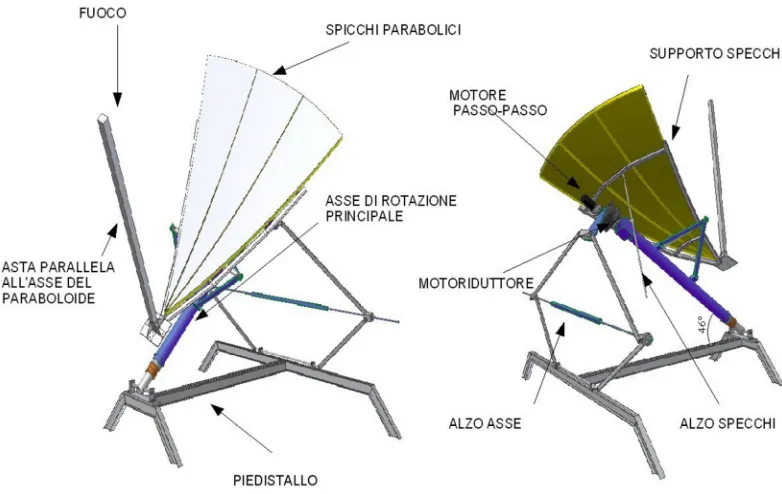
Presently the concentrator is made by three reflective parabolic sectors that can be disassembled and that have angular width of 15°; they are described in Paragraph 2.3. The overall prototype appears like in Figure 2.7. The apparatus is oriented with the x-y plane perpendicular to the incoming sunrays, and thus each sector has an ideal intercepting area of 0.818 m2.

2.4.1 Tracking

29

Figure 2.7: schematic representation of the concentrator prototype built at the University of Trento. Some components are shown: the parabolic sectors on the metal frame, the roll axis, the tilting screw, the stepping motor and the shaft supporting the receiver.

which is the main axis of tracking. The roll axis is placed in the north–south direction, and the elevation angle is such that the roll axis is parallel to the Earth axis (polar mount). This angle is of about 46°, as it is shown on Figure 2.7.

The tracking of the sun’s position is effected by a chronological tracker, which counteracts the Earth's rotation by turning at an equal rate as the earth, but in the opposite direction. Actually the rates aren't equal, because as the earth goes around the sun, the position of the sun changes with respect to the earth by 360° every year or 365.24 days. The drive method may be as simple as a gear motor that rotates at a very slow average rate of one revolution per day (15° per hour which corresponds to 0.00417°/sec).

Our tracking is achieved with a stepping motor Oriental Motor PK2913-E4.0T which needs about 400 steps to realize a full rotation. Two reduction mechanisms (Bonfiglioli) with reduction 1:10000 are connected to the stepping motor, resulting in a theoretical resolution of the tracking of 360°/(400K104) = 0.00009°. The main limitation to this is the mechanical play of the reduction mechanism.

2 Concentration PhotoVoltaic (CPV) systems

30

Figure 2.8: picture of the concentrator prototype. The image in the upper frame shows the illumination spot on the receiver.

31

2.5 Solar reflective modules

Concave mirrors are called "converging" because they tend to collect light that falls on them, refocusing parallel incoming rays toward a focus. We adopted silvered mirror as reflective material as it combines both high reflectance and good mechanical properties (Poullikkas et al., 2010). Compared with other mirror types, it is preferred for its high reflectance, good specularity, durability, and resistance to distortion from loads.

Despite these advantages, glass is heavy and brittle, requiring massive structural support (SERI, 1985). A good candidate as a structural material with proven rigidity under severe weather conditions is fiberglass. Fiberglass supports formed over a mandrel have been incorporated by Kansas Structural (Gill and Plunkett, 1997) and McDonnell Douglas (NREL, 1998).

2 Concentration PhotoVoltaic (CPV) systems

32

2.5.1 Manufacturing process

The dish, defined by Equation 2.15 and 2.16, has been ideally divided in 24 identical basic sectors (modules), every sector having angular width of 15° and 0.818 m2 nominal area normal to the z axis (net aperture area).

The process to manufacture the modules makes use of a mould made of resin. The lodging wall of the mould is convex and consists of a slice portion of a round paraboloid with upward-directed convexity. The mirror surface will acquire the shape of this wall, so great care must be applied in the refining of the mould. Each parabolic sector was manufactured by shaping a starting plane mirror and a support material in a unique process, resulting in a single composite piece with the desired curvature and continuous reflective surface. The first step to produce a module is the arrangement of a flat 0.8 mm thick silvered mirror (FAST GLASS®) onto the mould, with reflective surface turned towards said convex wall. Afterward, structural layers are deposited above the mirror in the following order: a fiberglass layer, a PVC panel and another fiberglass layer. An alternative module has been successfully produced by substituting the PVC panel with a parabolic-curved wood panel. Shaped thin still plates were inserted in the PVC panel to add stiffness to the whole structure and to help the maintenance of the curvature over time. This has been made in the wood panel, too, by previously curving some transversal and longitudinal fissures.

33

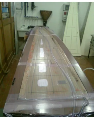
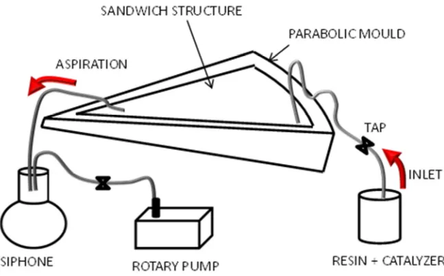
Figure 2.10: representation of the rosin infusion process.

The mould is then inserted inside a soft plastic bag connected to a rotary pump in order to create vacuum (see Figure 2.9). When an adequate vacuum (3 mbar) is reached, the difference from internal and external pressure is used as uniform force which shapes the layers against the mould surface. The same difference of pressure is used to insufflate into the fiberglass matrix a thermosetting epoxy resin; for such purpose, the non-rigid container is placed in communication, through an inflow line, with a resin tank (see Figure 2.10). The fluid resin, filling the non-rigid container, penetrates into the porous fiberglass and glues the stiff PVC layer to the mirror back-surface. The reduced pressure created inside the bag has the advantage of ensuring a gradual and uniformly distributed shaping of the mirror. A siphone has been placed at the end of the aspiration tube in order to protect the pump from resin contamination.

After about 14 hours the manufact is heated by means of warming stripes at ~70° for about 6 hours. The parabolic sector is extracted from the mould when the hardening of the resin, that requires some hours after the end of the infusion, is completed. More details about the different steps of the process are described in the patent [Bettonte et al., 2007].

2 Concentration PhotoVoltaic (CPV) systems

34

35

Chapter 3

Characterization of solar

collectors

3.1 Introduction

3 Characterization of solar collectors

36

In the first part of this chapter, Section 3.1, some characterization methods that have been used for concentrator photovoltaic applications are presented. Some of them have been adopted from other applications, since solar collector can be used for concentration solar application (CSP), too. Then the experimental work to evaluate the performance of our solar collector is reported. In particular we have measured the reflectance properties of the mirror material, the shape of the illumination profile e and the total power impinging on the receiver. To perform the last measurement a flat plate calorimeter was built and then a thermal balance study was carried out.

3.2 Optical

performance:

theory

and

testing

procedures

3.2.1 System preparation

The optical quality of an individual collector, which is part of a concentration photovoltaic system, is independent of the photovoltaic receiver used. In order to measure the performances of collectors, a two-axis solar tracker in which the collector–receiver is mounted and pointed to the sun, is required. The precision of its tracking and in the alignment of both the collector and light sensor will influence the capacity to characterize the collector, and it is independent from the optical quality of the collector itself. Before taking any measurement, the collector and the receiver have to be thoroughly cleaned.

3.2.2 Collector optical efficiency

The overall optical efficiency of the collector is defined as the ratio of the power incident on the receiver ($_LMN) to the power at its aperture plane ($ _O):

" #=$_$LMN

O =

PQ PRST

(3.1)

37

acceptance angle as that of the collector and P_Q is the average irradiance on the receiver; X_T is the geometric concentration, defined as:

ST= WN LMN

(3.2)

with _WN collector net aperture area and _LMNreceiver area.

The overall optical efficiency can be expressed as the product of two parameters:

" #= " #,TPX(Y) (3.3)

where PX(Y) is the global transmittance/reflectivity coefficient and refers to the intrinsic properties of the material of the collector, Y is the wavelenght, " _#,T is the geometric optical efficiency depending on the collector geometry and characteristics, especially relating its shape, including the losses not included in PX(Y). The micro-imperfection of a reflective surface are mainly contained in PX(Y), whereas the macro imperfections impact " _#,T.

The parameter PX(λ) depends on the material transmittance or reflectivity characteristics and includes losses due to the material absorption and losses caused by the spectral modification of the solar light at the collector. It is obtained from the following equation:

PX[YH, Y ] =\ ](Y)X(Y)^Y _`

_a

\ ](Y)^Y_` _a

(3.4)

where ](Y) is the spectral distribution of light falling on the collector; X(Y) is the spectral transmittance/reflectivity of the unshaped material. " _# depends on the radiation wavelength range [λ_H, λ ] trough PX(Y). In order to evaluate PX(Y), the X(Y) coefficient must be known, and its meaning and evaluation procedure are different for specular collectors or lenses. Radiation falling on the collector aperture plane GI must be measured with a sensor with the same angular acceptance as the concentrator to be characterized. Two cases can be observed.

3 Characterization of solar collectors

38

the diffuse radiation coming from the sky. The incoming radiation is measured with a pyrheliometer having an acceptance angle within 5°. Thus

PR= g (3.5)

where g is the direct irradiance measured with the pyrheliometer.

2. Systems with angular acceptance higher than 5°, can collect direct irradiance and some of the diffuse irradiance coming from the sky. If no specific measurement system with the same acceptance is available, incoming radiation can be calculated from the measurements obtained by means of a pyrheliometer and a pyranometer. Thus way

PR = g 2 h( (3.6)

where ( = P − g is the diffuse irradiance calculated from direct radiation g, measured with the pyrheliometer, and P is the global radiation, measured with the pyranometer; h is the fraction of collected diffuse radiation, evaluated according to the acceptance angle of the collector. In order to measure the radiation spectral distribution ](Y), necessary to separate the optical efficiency losses of geometry and shaping " _#,T, from those of the material PX(λ), a portable spectrometer is needed. From the measurement, this distribution results as:

]R(Y) = PRkR(Y) (3.7)

where

\ k_{_}__`a R(Y)^Y = 1; (3.8)

]R(Y) is the absolute spectral distribution (W cm-2 nm-1) and kR(Y) is the relative spectral distribution (nm-1).

3.2.3 Intercept factor

39 m =Onop

Onoq. (3.9)

Its value depends on the size of the receiver, the surface angle errors of the parabolic mirror, and solar beam spread. The errors associated with the parabolic surface are of two types, random and non-random. Random errors are identified as apparent changes in the sun's width, scattering effects caused by random slope errors (i.e. distortion of the parabola due loading) and scattering effects associated with the reflective surface, and can be represented by normal probability distributions. Non-random errors arise from the manufacturing process and/or from the assembling of the optical elements and/or from the pointing or tracking of the collector. These errors can be identified as reflector shape imperfections, misalignment errors and receiver location errors. Random errors are modeled statistically, by determining the standard deviation of the total reflected energy distribution, at normal incidence [Guven and Bannerot, 1986] as specified in equation 3.9:

s = t s A 2 4 s Au # 2 s (3.10)

where σ_wxy is the standard deviation of the energy distribution of the sun's rays at normal incidence, σ_wz{|} is the standard deviation of the distribution of local slope errors at normal incidence, and σ_9•=={= is the standard deviation of the variation in reflectivity of the mirror at normal incidence.

Non-random errors are determined from the knowledge of the misalignment angle error € (i.e. the angle between the reflected ray from the center of sun and the normal to the reflector's aperture plane) and of the displacement of the receiver from the focus of the parabola (^0).

3 Characterization of solar collectors

40 γ=1 2 cosφ

2 56 φ ƒ „ … † … ‡ ]0, ˆ ‰ Š

‹56 φ Œ(1 2 345φ)(1 − 2 ^∗56 φ) − πβ∗(1 2 cosφ )

√2πs∗(1 2 cosφ )

• • ‘ φ ’ −]0, ˆ ‰ Š

‹56 φ Œ(1 2 345φ)(1 2 2 ^∗56 φ) 2 πβ∗(1 2 cosφ )

√2π s∗(1 2 cosφ )

• • ‘ “ … ” … • ^φ (1 2 345φ)

(3.11)

where φ is the collector rim angle (degrees), s∗ is the universal random error parameter (s∗= s ) and β∗ is the universal non-random error parameter due to angular errors (β∗=β ).

3.2.4 Solar mirror reflectance

41 Figure 3.1: Definition of angles.

The specular reflectance —_š(Y, , –) is measured with a specular reflecto-meter at = 3.5, 7.5, and 12.5 mrad with an incidence angle – = 15° for Y ≈ 660 h. For highly specular reflectors, specular reflectance can then be described by the ratio of specular reflectance —_š(Y, , –) to the hemispherical reflectance —_˜(Y, , –) at the same wavelength; this ratio is assumed to be constant and equals the ratio of the solar weighted values. The solar-weighted specular reflectance is then approximated by [Pettit, 1982]:

—š‹ρ_A ,φ,θŒ = —š(Y = 660 h,φ,θ )

—š(Y = 660 h,φ,θ ) K —˜‹ρA ,φ,θŒ

(3.12)

3.2.5 Distribution of concentrated light at the receiver

The quality of a collector depends not only on its optical efficiency, but also on the distribution of light on the receiver. In fact, the spot light profile produced by the collector is fundamental to the design of the system. The size of the receiver is usually chosen a priori and is based on technological and economic considerations. On the one hand, the materials chosen affect the optical efficiency through the global transmittance/reflectivity coefficient parameter (PX, equation 3.3), that can be taken equal to the solar-weighted specular reflectance —> (ρ_A , , –) for solar reflectors; on the other hand, the ability of the manufacturing process to reproduce the theoretical reflective surface determines the distribution of the energy on the receiver and thus

Incident

beam

Normal

Specular

reflected

beam

Scattered

reflection

φ θ

3 Characterization of solar collectors

42 affects the optical efficiency, too.

A tool for measuring the light distribution produced by the collector, therefore, will serve not only to compare manufacturing processes and give the information for designing the receiver, but also to determine the efficiency of the system for a certain concentration level. It is possible that a collector designed for a relatively high concentration level has poor optical quality as a great part of the light falls outside the receiver for which it was designed; at lower concentrations the optical quality in general is higher.

The measurement of concentrated solar flux can be made with radiometric methods, through thermocouples, thermopiles, or photo-sensors and it requires calibration. In [Chong et al., 2011] an optical scanner based on a photodiodes array capable of plotting the flux distribution has been proposed, with the advantage of performing real time and direct measurement of very high-concentrated fluxes without the risk of burning the diffuser.

In spite of this, thanks to its high resolution, the most common procedure to measure the irradiance distribution make use of a CCD camera and a receiver placed in the focusing region of the collector [Parretta et al., 2006; Johnston, 1998]. The collector and the receiver have to be positioned on a two-axis tracker with the camera moving in line with them. In case of high irradiance values, a set of filters are needed in order not to saturate the image obtained. A lambertian plane surface (the angular distribution depends on 345 –, where – is the angle to the perpendicular) is used as a receiver. In this way all the radiation coming from the mirror is collected equally, and given that the object is to take a measurement relative to the distribution of the light, the angle at which the camera sees the reflector has no influence. Differently, if the receiver behaved as a reflector, the light power detected by the camera would correspond to a fraction of the mirror area and not to its totality, falsifying the measurement. A lambertian receiver can be obtained with a flat microgranular surface painted matt white.

43

possible solution is to place the CCD camera behind a lambertian diffuser, in transmittance configuration. The CCD camera provides a matrix of pixels I (i, j), which contains the irradiance level for each pixel, whose coordinates are (i, j). The measurements obtained through this process are always relative, although a calibration the system can be carried out in order to find out the absolute value of the irradiance in W/cm2 [Ulmer et al., 2002].

Figure 3.2: Different system configuration in order to measure the light distribution for different solar collectors: (a) linear, (b,c) parabolic dish.

3.2.6 Calorimetry

3 Characterization of solar collectors

44

carry out this task [Gardon, 1953; Pérez-Ràbago et al., 2006]. The disadvantage of these methods is that all radiometers require calibration, and this is not easy due to spectral response effects.

Calorimeters are used to measure the concentrated flux in a direct way. A device of this type allows exchanging the power produced by the pointed-to-sun concentrator module with a heat transfer fluid, usually water, flowing through the calorimeter body. The incident concentrated flux can be evaluated by determining the heat absorbed by fluid and estimating the external heat losses. This technique requires reducing to a minimum the uncertainties in the measurements of the mass flow rate of the cooling fluid, and of the difference between its inlet and outlet temperatures. One of the calorimetric techniques that have been successfully explored is the Cold Water Calorimetry (CWC) [Buck et al., 2002]. Here very good heat transfer from the concentrated flux to the fluid flow is needed, in order to have the receiving surface of the calorimeter at a temperature close to ambient. This can be achieved by increasing the fluid flow rate. In this way is possible to reduce radiative and convective losses, hopefully eliminating the need for a precise estimation of these losses.

3.3 Experimental

45

high-flux solar energy arriving at the focus of a module, a flat-plate calorimeter was built. The study was carried out by measuring the energy absorbed by the water flow and the external losses due to convection. Based on an energy balance, the intercept factor and the overall optical efficiency of the collector were estimated.

3.3.1 Measurement of reflectance of silvered mirrors

The reflectivity of an ideal (front-surface) silvered mirror is approximately 97%. Since silver degrades quickly in the outdoor environment, more durable back-surface glass mirrors have typically been used at CSP and CPV plants. Glass superstrates result in transmission losses (increased absorption) through the glass medium, with losses increasing as a function of both iron content in the glass and thickness. The reflectivity of typical mass-produced commercial glass exhibit lower reflectivity, ≤90%, due to increased absorption and thickness.

We have used a 0.8 mm thick silvered mirror produced by FAST GLASS® whose reflectivity properties have to been assessed. Microscopic surface irregularities, called specularity errors, in a mirror’s substrate or superstrate material slightly reduce a mirror’s measured specular reflectivity because they cause non-specular (scattered) reflections that fall outside the acceptance aperture of the measurement instrument. Specularity errors can be measured on small mirror samples and generally have a much smaller impact on plant performance than “slope” and “curvature” errors, which are errors in the shape of the mirror surface over larger macroscopic areas of the surface that must be measured on full-size samples.

3 Characterization of solar collectors

46

(Varian Cary 5000) as a function of the wavelength of the incident radiation. The acquisition has been made over a wavelength range λ = 250-1200 nm of the scanning radiation and with a fixed incident angle θ =12.5°. The spectrophotometer was equipped with a PMT detector (250 – 800 nm) and with a PbS detector (800-1200 nm). The measured reflectance R(λ) is shown in Figure 3.3. It holds 93.0% ± 0.1 % for

λ > 500 nm, reaching a maximum value of 94.4% ± 0.1 % around 700 nm. At low wavelength values the reflectance decreases to 89.8% at around 465 nm and falls below 80.0 % at 426 nm and below 70 % at 395 nm.

Figure 3.3: reflectance curve R(λ) of the unshaped silvered mirror measured with a UV-Vis spectrophotometer.

47

surface absorption is almost insensitive to the spectral content of the incoming radiation. Differently, if the mirror is used in a Concentration PhotoVoltaic (CPV) application, spectral variations have to be carefully considered. This is particularly true when multijunction cells are the active elements of the receiver, because each

sub-cell thickness is designed to satisfy current-matching requirements, that depends upon the spectral distribution of the incident light. The sensitivity of MJ devices to variable spectrum has been studied theoretically [Kurtz et al. 1990], but not yet experimentally to our knowledge.

In our case the reflective material acts as a filter for wavelengths below 400 nm, so it would have an influence on the electrical behavior of every cell that has been

Figure 3.4: standard AM1.5 direct solar spectrum (ASTM G173-03 D) and the same spectrum after reflection by the silvered mirror (ASTM G173-03 DR). This last curve was calculated by using the reflectivity curve shown in Figure 3.3.

3 Characterization of solar collectors

48

measurement of this parameter. This procedure has the advantage to give an effective value that describes the performance of the mirror material at a given solar radiation condition. The measurement has been carried out with respect to the solar spectrum incident at a given angle of θ = 45° and along a series of 20 repetitive measurements within half an hour. For this purpose a device supporting a piece of plane mirror and a pyroheliometer, accurately aligned by means of a laser-pen, has been mounted on the solar tracker. The sunlight incident on the mirror at 45° is reflected to the entrance aperture of the pyroheliometer, having an aperture cone φ = 5°.

This way we can define an effective value for solar-weighted reflectance as:

—•• =$_$’ (3.13)

where P_• is the incident solar power measured by the pyroheliometer and P_’ is the power measured after a reflection on the mirror's surface. Power values were measured with the same pyroheliometer, by pointing it alternatively to the sun and to the mirror's output beam. The resulting value for — _•• was 89.6 % with a standard deviation of 0.4%. It must be emphasized that this value refers to an incident angle of the sunlight on the plane mirror of 45°, with respect to the rays coming from the center of the solar disk.

When this solar-weighted reflectance — _•• is used as a figure of merit for our oriented parabolic sector, the dependence of RS from the angle of incidence θ is neglected. The angle of incidence θ on the oriented sector ranges between 0° (incident solar rays near the vertex of the sector) and 64° (incident rays on the largest side of sector).

3.3.2 Illumination profile measurement

49

representative points by using an electrical plotter with x and y movements (Micos) and a powermeter (Ophir Ltd), as it is shown in Figure 3.5. The thermal head (Ophir F150A), which allows to measure average power density up to 15 kW/cm2, was mounted upon the plotter and was connected to an Ophir Vega display and to a computer. To enhance the spatial resolution of the power density measurement, the 17.5 mm diameter of the thermal head was protected with a water cooled copper shield, with an aperture hole whose area was measured to be 16.66 ± 1.44 mm2.

Figure 3.5: experimental apparatus used to scan the illumination profile, mounted on the sun tracking system.

3 Characterization of solar collectors

50

equal to the instantaneous direct solar radiation express in W/m2. Solar radiation was measured with a calibrated pyroheliometer (Kippen&ZonenCHP1). Figure 3.6 (left) shows the radiative flux distribution at the focal region in terms of power density units (W/cm2), as a result of the interpolation of experimental data. The spot shape is close to a Gaussian distribution with a mean power gradient of about 2.23 W/(cm2mm) and a peak flux of 73 W/cm2, corresponding to a peak concentration ratio of about 870 X.

The spot measured at 2460 mm is shown in Figure 3.6 (right). The mean power value of the direct solar radiation during the acquisition time was 831 W/m2. In this case the spot loses its symmetry, the illuminated area becomes larger and the peak flux lower (62 W/cm2).

51

Figure 3.7: calculated 3D profile and ‘contour plot’ of the density power for a parabolic module. The image is referred to power density expected on a plane perpendicular to the z axis of the paraboloid, at a distance of 2500 mm from the origin plane. The collector is considered and having no surface errors and a weighted-solar spectrum reflectivity of 0.876. Values reported on the contours are expressed in W/cm2.

In Figure 3.7 is reported the flux distribution simulated with a Monte Carlo (MC) ray-tracing technique. Simulation was performed with a reflector having no surface errors (zero slope error) and in nearly the same conditions of the reflector under testing: same shape, sizes, solar-weighted reflectance of 0.896, as estimated in the previous paragraph, and incident direct solar radiation of 835 Wm-2. A sample of 106 sunrays/m2 in the MC run, and the sunshape model with circumsolar ratio CSR=5% were used [Buie et al, 2003]. In this case the spot is smaller and the peak reaches values of about 110 W/cm2.

3 Characterization of solar collectors

52

Figure 3.8: measured and calculated power fraction collected in circles of radius R at the focal plane of the parabolic sector.

3.3.3 Calorimetric measurement

The aim of this work is to determine the solar energy concentrated by a parabolic module onto the spot region. To achieve this goal is necessary to quantify the global heat losses to the environment, thus establishing the validity of the Cold Water Calorimetry (CWC) for the system. In order to keep the design of the calorimeter as simple as possible, a flat plate device has been built (Jaramillo et al., 2007). In this type of calorimeter concentrated sun rays hit a plate receiver and part of the light is back-reflected. These losses are greatly higher than in a cavity calorimeter (in which the sun rays are reflected inside the cave), but at the same time they are easier to estimate. In order to increase solar absorption, the receiving face of the calorimeter has been chemically oxidized.

Part of the energy absorbed by the calorimeter is lost towards the environment through convective and radiative heat transfer. To calculate this portion of energy, the temperature of the front face of the calorimeter has to be accurately measured.

Description of the calorimeter

53

oxidized to increase the solar absorption; the rear part has been carved into channels and then covered with a thin copper plate (3 mm), which has been soldered to the body. The section of the channels is a 5 by 5 mm square, while the walls between the channels are 3 mm thick. Water enters from the back of the plate, near the center, flows through the channels alternating clockwise and counterclockwise direction and finally exits near the edge. Along this path, water increases its temperature, subtracting heat from the copper plate. The channels’ function is to force the water to keep a steady velocity in the rear part of the plate, avoiding the formation of vortexes and stagnation.

In the walls that separate the channels, 13 holes, 9.5 millimeters deep and horizontally lined up, have been drilled. These holes host 13 type-k thermocouples,

Figure 3.9: exploded representation of the calorimeter. The 12 thermocouples and the insulating material are not drawn.

which directly measure the temperature of the front plate, which will then be used to calculate convection losses.

The sides and the back of the plate have been insulated with 6mm thick pyrogel STEEL CASING

CHANNELS FRONT FACE

WATER INLET

AND OUTLET THERMOCOUPLES

3 Characterization of solar collectors

54

6671, an insulation blanket formed of silica aerogel and reinforced with a non-woven, glass-fiber batting. The insulated copper plate is contained into a stainless still, which can be easily fixed to our concentration solar collector. Thermal conductivity of

pyrogel is less than 18 mW/(m·K) under 100°C

[ http://www.teknowoolnanotecnologie.com/documenti/Aspen/Scheda%20tecnica %2 0Pyrogel_6671.pdf] which is the range of temperature we expect to reach on the front face. This low conductivity layer allows to disregard thermal losses toward the steel stand, and only consider losses from the front face (reflection, convection and radiation). A more detailed description of the calorimeter sub-components is given in Appendix A.

Oxidation process

To obtain a high absorption surface, the copper has been oxidized through a chemical treatment. First, the plate has been lapped with different grade silicon carbide papers; further degreasing was then obtained by dipping it in Rodaclean supra solution (5%) for 3 minutes at 60°C; finally the surface oxide has been removed with a 1% HCL solution. The cleaned copper plate was then immersed into a sealed glass container, containing an alcaline solution (0.1M NaOH) of K2S2O8 (0.001M). In this condition,

the plate was left still at 70°C for 16 hours. Such oxidation of copper normally proceeds through the precipitation of copper oxide salt on the surface, which then

decomposes to produce copper oxide film. After reaction, the sample was taken out,

washed with distilled water and dried in air. A dark film was obtained,which covered

uniformly the copper substrate.

55

Figure 3.10: diffuse reflectivity of the copper oxide layer (yellow) with respect to the reference Teflon sample (blue). The ASTM G173-03 solar spectrum is also shown (green).

Physical process

When direct sunlight is collected by the parabolic module, part of it is reflected in the focus region and the rest is scattered or absorbed by the glass layer. In case of an ideal dish collector of collecting area, the fraction

$ u = —š% (3.14)

would hit the plate of the calorimeter, where —_š is the solar-weighted specular reflectance of the mirror and % is the direct solar intensity. In case of a real solar collector, an energy balance on the copper disc has to be carried out in order to determine the impinging high-flux solar energy. Neglecting the losses from the back and lateral faces of the calorimete