Fault Diagnosis of Rolling Bearing Based on Tunable
Q-Factor Wavelet Transform and Convolutional Neural
Network
https://doi.org/10.3991/ijoe.v16i02.11953
Liqun Hou (), Zijing Li
North China Electric Power University, Baoding, China [email protected]
Abstract—The rolling bearing plays is used extensively in rotary machines
and industrial processes. Effective fault diagnosis technology for a rolling bear-ing directly affects the life and operator safety of the device. In this paper, a fault diagnosis method based on a tunable-Q wavelet transform (TQWT) and a convolutional neural network (CNN) is proposed to reduce the influence of noise on the bearing vibration signal and to reduce the dependence on human experience in traditional diagnosis methods. TQWT is used to decompose and denoise the vibration signal, while the CNN extracts fault features and per-forms fault classification. Seven motor operating conditions—normal, drive end rolling ball failure (DE-B), drive end inner raceway failure (DE-IR), drive end outer raceway failure (DE-OR), fan end rolling ball failure (FE-B), fan end in-ner raceway fault (FE-IR) and fan end outer raceway fault (FE-OR)—are used to evaluate the proposed approach. The experimental results indicate that the fault diagnosis accuracy of the proposed method reaches 99.8%.
Keywords—Fault diagnosis, tunable Q-factor wavelet transform, convolutional
neural network, rolling bearing
1
Introduction
Rolling bearings are widely employed in many machines. Its operational condition directly influences the lifetime and operator safety of the machine. Effective condition monitoring and fault diagnosis on rolling bearings are able to prevent unexpected device faults and enhance device operational efficiency [1-2]. Currently, there are two main categories of rolling bearing fault diagnosis techniques.
the noisy vibration signals of rolling bearings. The experimental results indicate that the proposed approach is more suitable for the incipient fault detection compared with the traditional signal denoising methods. Manjurul et al [5] presented a bearing fault diagnosis approach using bearing acoustic emission signals and a Bayesian inference-based multi-class support vector machine, and the proposed method is able to improve the classification accuracy. Tiwari et al [6] proposed a bearing fault diagnosis method using multi-scale permutation entropy and an adaptive neuro fuzzy classifier, and the experimental results verify the potential application value of their method for early bearing fault diagnosis.
In summary, the first category of bearing fault diagnosis methods is able to obtain acceptable fault diagnosis results. However, it depends mainly on previous experience to extract surface fault features, and it cannot deeply mine the correlation between vibration signal and bearing fault types. Moreover, the signal proceeding methods and pattern recognition methods are combined randomly in most application cases in this category. These drawbacks limit the broader application of these techniques.
The second category uses deep learning to extract fault features and realize fault classification. Since Hinton put forward the concept of deep learning [7], it has been successfully applied in many fields such as data transmission in IoT [8], image classi-fication [9], and language understanding [10]. Several deep learning approaches have also been developed and reported for fault diagnosis. Xu et al [11] proposed a bearing fault diagnosis method by using a deep belief network with multiple hidden layers and affinity propagation. This method eliminates the dependence of fault labels on train-ing processes and improves the efficiency of traintrain-ing. Compared with the traditional empirical mode decomposition methods, it has higher fault diagnosis accuracy. So-haib et al [12] combined a hybrid feature pool and a deep neural network based on sparse stacked autoencoders (SSAEs) to identify different bearing faults and their severities. The experimental results show that compared with support vector machines and back propagation neural networks, the presented method can better classify bear-ing defects with various severities. Sun et al [13] proposed an intelligent bearbear-ing fault diagnosis approach based on compressed sensing and a SSAEs-based deep neural network to reduce the computing workload for processing the massive fault data. The effectiveness of the method is verified by rolling bearing data sets from Case Western Reserve University Bearing Data Center.
convolu-tional neural network and wavelet packet transform to automate and better generalize the fault feature extraction and diagnosis process. Experimental results show that the presented method outperforms the existing multi-fault classification algorithms and has good classification accuracy.
The wavelet is a famous tool for signal and data processing. Since last year, re-searchers began to combine wavelet with CNN for various applications. Discrete wavelet transforms (DWT) and CNN were successfully used to identify gearbox faults [18], facial expressions [19], and brain tumors [20], while continuous wavelet transform (CWT) and CNN were explored to detect feeder faults in resonant ground-ing distribution systems [21]. In addition, wavelet packet decomposition (WPD) and CNN were successfully employed to build the wind speed prediction model [22].
The tunable-Q wavelet transform (TQWT) was proposed by Selesnick in 2011. Compared with the wavelet transform and Fourier transform, the TQWT is more suit-able for analyzing nonstationary signals [23]. Although, there have been several suc-cessful applications of bearing fault diagnosis by using TQWT [24], bearing fault diagnosis by combining TQWT and CNN is a relatively unexplored area.
Compared with the above bearing fault diagnosis methods, this paper proposes a novel fault diagnosis method based on TQWT and CNN, in which TQWT is used to eliminate the influence of noise on original bearing vibration signal, while CNN is adopted for fault diagnosis.
The remainder of this paper is organized as follows. The principles of TQWT and CNN are briefly introduced in Section II. Section III describes the implementation methodology and gives the experimental results. Finally, Section IV presents the overall conclusions.
2
Theoretical Background
2.1 TQWT principle
TQWT is a fully discrete wavelet transform implemented by the iteration of two-channel filter banks and a discrete Fourier transform. Different from the traditional wavelet transform, TQWT is based on the oscillatory behavior of the measured signal rather than frequency behavior of the signal, and can adaptively adjust the Q value of the wavelet basis function according to the signal characteristics. Therefore, the de-grees of oscillation in the wavelet basis function and in the extracted components of the measured signal can be better matched by using TQWT [23-26].
Q-factor (𝐐): The Q-factor (denoted as 𝑄) of the TQWT is defined as
𝑄 = 𝑓𝑐
𝐵𝜔 (1)
where 𝑓𝑐 is the center frequency of the signal and 𝐵𝜔 is signal bandwidth. It can be
oscilla-tory signal with large bandwidth, while a low Q-factor is appropriate for little or no oscillatory behavior with small bandwidth.
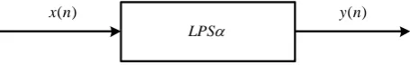
Low-pass scaling: The low-pass scaling in the frequency domain preserves the low-frequency content of the signal. The principle of low-pass scaling is shown in Fig.1. 𝛼 is the low-pass scaling parameter. If the sampling frequency of the input signal is 𝑓𝑠, the sampling frequency of the output signal will be 𝛼𝑓𝑠.
Fig. 1. Block diagram of low-pass scaling
High-pass scaling: The high-frequency content of the signal is preserved with high pass scaling. The block diagram of the high-pass scaling is illustrated in Fig. 2. 𝛽 is the high-pass scaling parameter. If the sampling frequency of the input signal is 𝑓𝑠, the
sampling frequency of the output signal will be 𝛽𝑓𝑠.
Fig. 2. Block diagram of high-pass scaling
The high-pass and low-pass scaling parameters are defined as
𝛽 = 2
𝑄+1𝛼 = 1 − 𝛽
𝛾 (2)
Where 𝛾 is the redundancy factor that is usually no less than 3. To prevent the over redundancy of the wavelet transform and obtain perfect reconstruction with TQWT, both 𝛼 and 𝛽 should satisfy0 < 𝛼 < 1, 0 < 𝛽 < 1, and 𝛼 + 𝛽 > 1.
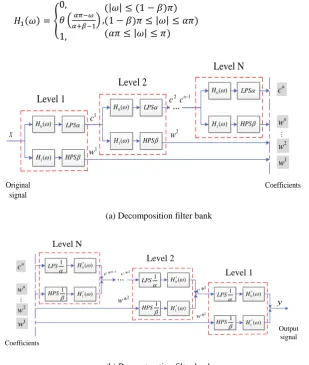
Signal decomposition and reconstruction: When the measured signal is pro-cessed by TQWT, the signal is decomposed and reconstructed by iteratively using the decomposition filter bank and reconstruction filter bank. Taking an N-layer signal decomposition and reconstruction as an example, the corresponding dual-channel filter banks are illustrated as Fig. 3.
𝐻0(𝜔) and 𝐻1(𝜔) are the frequency response functions of the low-pass filter and
the high-pass filter, respectively, while 𝐻0∗(𝜔) and 𝐻1∗(𝜔) are the complex conjugates
of 𝐻0(𝜔) and 𝐻1(𝜔).𝐻0(𝜔) and 𝐻1(𝜔) are generally defined as
𝐻0(𝜔) = {
1,
𝜃 (𝜔+(𝛽−1)𝜋
𝛼+𝛽−1 ) ,
0,
(|𝜔| ≤ (1 − 𝛽)𝜋) (1 − 𝛽)𝜋 ≤ |𝜔| ≤ 𝛼𝜋) (𝛼𝜋 ≤ |𝜔| ≤ 𝜋)
(3) ( )
x n y n( )
LPS
( )
x n y n( )
𝐻1(𝜔) = {
0, 𝜃 (𝛼𝜋−𝜔
𝛼+𝛽−1) ,
1,
(|𝜔| ≤ (1 − 𝛽)𝜋) (1 − 𝛽)𝜋 ≤ |𝜔| ≤ 𝛼𝜋) (𝛼𝜋 ≤ |𝜔| ≤ 𝜋)
(4)
x
0( )
H LPS
0( )
H LPS
...
0( )
H LPS
1( )
H
1( )
H
1( )
H HPS HPS HPS
Level 1
Level 2
Level N
Original signal 1 c 2 c n c 1 w 2 w n w 2 w 1 w 1 n c ... Coefficients(a) Decomposition filter bank
... 1 LPS 1 LPS 1 LPS * 0( ) H
* 0( ) H *
0( ) H
* 1( ) H
* 1( ) H *
1( ) H 1 HPS 1 HPS 1 HPS Level N Level 2 Level 1 y Output signal 1 * c 2 * c 1 *n c 1 * w 2 * w n c 1 w 2 w n w ... Coefficients
(b) Reconstruction filter bank
Fig. 3. N-level TQWT based on (a) decomposition filter bank and (b) reconstruction filter bank
Where 𝜃 is the Daubechies frequency response with two vanishing moments that are defined as =1
2(1 + 𝑐𝑜𝑠 𝜔)√2 − 𝑐𝑜𝑠 𝜔 , 𝜔 ≤ 𝜋. To obtain perfect reconstruction,
𝐻0(𝜔) and 𝐻1(𝜔) should satisfy |𝐻0(𝜔)|2+ |𝐻1(𝜔)|2= 1.
The frequency response of TQWT is filter banks with non-constant bandwidth. The adjacent frequency bands of TQWT are non-orthogonal. Let J denote the level of TQWT subbands, the center frequency 𝑓𝑐 and bandwidth 𝐵𝜔 of the frequency
re-sponse producing subband J can be approximately calculated by
𝑓𝑐= 𝛼𝐽 2−𝛽4𝛼 𝑓𝑠 (5)
𝐵𝜔 = 1
2𝛽𝛼
The length of the measured signal determines the number of TQWT levels, and the theoretical maximum decomposition level of TQWT is given by
𝐽𝑚=
⌊
𝑙𝑜𝑔( 𝑁 4𝑄+1)
𝑙𝑜𝑔( 𝑄+1 𝑄+1−2𝛾)⌋
(7)
where 𝑁 is the length of the measured signal to be decomposed, and ⌊∙⌋ represents the rounding function.
TQWT can set its Q-factor according to the actual applications without relying on the basis function. All the wavelets based on the same basis function and different Q-factor and the redundancy Q-factor 𝛾 built up a library of wavelet functions. Therefore, TQWT is essentially a constant Q-factor wavelet transform with a certain degree of redundancy.
2.2 CNN principle
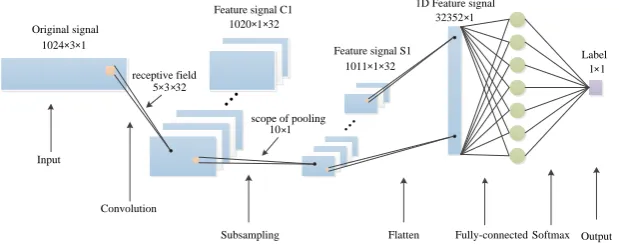
Generally, a CNN consists of an input layer, multiple alternating convolutional layers (i.e. C1…Cn) and pooling (sub sampling) layers (i.e. S1…Sn), a fully connected layer, and an output layer. In this research, one convolutional layer and one pooling layer are employed. The architecture of the CNN used in this application is depicted in Fig. 4.
Input
Convolution
...
...
Subsampling Flatten Fully-connectedSoftmax Output 1024 3 1
1020 1 32
1011 1 32
32352 1
5 3 32
10 1
1 1
×
× ×
× ×
×
×
× ×
×
×
receptive field
scope of pooling Original signal
Feature signal C1
Feature signal S1
1D Feature signal
Label
Fig. 4. Convolutional neural network structure
Input layer: In this paper, the input of the CNN is the vibration signal of the roll-ing bearroll-ing operatroll-ing at various conditions. The size of the input data is 1024×3×1. Every data set consists of 1024 sampled points and every sampled point includes three vibration data obtained from the drive end, the fan end and the base of the motor.
Convolutional layer: The convolutional layer extracts the features of the original vibration signal. When the vibration signal is input to the CNN, a convolution opera-tion with each receptive field is carried out using
𝐻𝑗= 𝑓(∑ 𝐻𝑖′× 𝑊𝑖𝑗+ 𝑏𝑗 𝑝
where, 𝐻𝑗 is the j-th output feature map of current layer, 𝐻𝑖′ is the i-th output
fea-ture map of the previous layer, 𝑊𝑖𝑗is the weight matrix connecting the 𝐻𝑖′ and 𝐻𝑗, 𝑏𝑗is
the additive bias of the j-th receptive field, and 𝑝 is the number of receptive fields in the previous layer.
Before training the CNN, the size and number the receptive field are set at 5×3 and 32. The output after the convolution of the vibration signal and the receptive field is feature signal C1.The number of channels is consistent with the number of receptive fields, and its length and width are ℎ′ and 𝑤′ respectively. ℎ′ and 𝑤′are given by
ℎ′= ⌊ℎ−𝑚+𝑠
𝑠 ⌋ 𝑤
′= ⌊𝑤−𝑛+𝑠
𝑠 ⌋ (9)
where, ⌊∙⌋ represents downward rounding, ℎ and 𝑤 are the length and width of the input data, while 𝑚, 𝑛, and 𝑠 are the length, width, and stride length of the receptive field, respectively.
In this example, the ReLU function is used as the activation function. The dimen-sion of feature signal C1 is unchanged by the activation function, so the size of feature signal C1 is 1020×1×32.
Pooling layer: Pooling layers reduce the dimension of extracted features to obtain the most essential signal features. Feature signal C1 is the input of the pooling layer, and feature signal S1 is the output of the pooling layer. The calculation formula for the pooling layer is
𝐻𝑗= 𝑓(𝛽𝑗𝑑𝑜𝑤𝑛(𝐻𝑗′) + 𝑏𝑗) (10)
Where, 𝐻𝑗 is the j-th output feature signal of current layer, 𝐻𝑗′ is the j-th output
fea-ture signal of the previous layer, 𝑑𝑜𝑤𝑛(∙) represents pooling rules, 𝛽𝑗 is the j-th
mul-tiplicative bias of current layer, and 𝑏𝑗 is the j-th additive bias of current layer.
In this case, maximum pooling with a range of 10×1 and a stride length of 1 is adopted. The dimension calculation method of feature signal S1 is similar to equation (10). As the pooling calculation only changes feature signal size, the dimension of feature signal S1 is 1011×1×32.
Fully connected layer and output layer: Through expanding the feature signal S1, a 1D Feature signal with a dimension of 32352×1 is obtained, which is used as the input signal of the fully connected layer. In this paper, the CNN is used to classify seven motor operating conditions network, so the fully connected layer has seven receptive fields and the size of the fully connected layer is 32352×1. The fully con-nected layer is calculated by
𝑦 = 𝑓(𝑊𝑇𝑥 + 𝑏) (11)
3
Experimental Validation
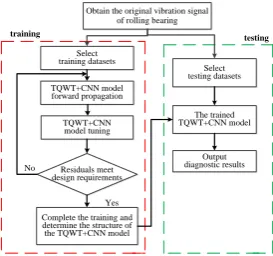
The flowchart of the proposed rolling bearing fault diagnosis approach based on TQWT and CNN is shown in Fig. 5. It consists of a training part and a testing part. The training part implies the following steps.
Firstly, the Q-factor and redundancy γ are determined according to the original vi-bration signal characteristics and empirical methods, respectively, and then the opti-mal decomposition layers J are found.
Secondly, the vibration signal is decomposed and denoised using the TQWT with the selected parameters from the previous step.
Thirdly, the CNN is trained and tuned using the vibration signals processed by TQWT to obtain the essential fault features. Finally, the mapping relationship be-tween the output of CNN and the corresponding bearing faults are determined. In the testing part, when the testing data sets are input the TQWT and CNN models obtained from the training data, the diagnosis results are obtained.
The algorithms implementing the flow chart of Fig. 5 are coded using MATLAB on a laptop with Intel i3-3240 3.4GHz CPU and 8GB RAM. As this paper mainly explores the feasibility of fault diagnosis using TQWT and CNN, instead of building up a testbed, this paper directly uses the data released by the Case Western Reserve University Bearing Data Center [27]. The experimental setup includes a 2hp electric motor, a torque sensor, a power test meter, a controller, and three accelerometers recording the vibration signals at the base plate, the drive end and the fan end of the motor.
In this experiment, seven motor operating conditions, normal, drive end rolling ball failure (DE-B), drive end inner raceway failure (DE-IR), drive end outer raceway failure (DE-OR), fan end rolling ball failure B), fan end inner raceway fault (FE-IR) and fan end outer raceway fault (FE-OR), were used to evaluate the feasibility of the proposed diagnosis method. The size of the fault is 7 mils and the signal sampling frequency is 12 kHz. 700 sets of vibration data, 100 sets for every operating condi-tion, are used in this research. Every data set consists of 1024×3 samples, namely the vibrations at the base plate, the drive end and the fan end of the motor.
Obtain the original vibration signal of rolling bearing
Select training datasets
TQWT+CNN model forward propagation
TQWT+CNN model tuning
Complete the training and determine the structure of the TQWT+CNN model
Residuals meet design requirements
Select testing datasets
The trained TQWT+CNN model
Output diagnostic results No
Yes
training testing
3.1 Signal denoising by TQWT
In order to reduce the influence of noise on the fault diagnosis result, the original vibration signal is firstly denoised by TQWT. The choice of the redundancy 𝛾 of TQWT is limited by the high and low filter transform scales, so the value of redun-dancy must be strictly greater than 1. But when the redunredun-dancy is too small (i.e., close to 1), the frequency domain response bandwidth of the signal is narrower, resulting in local degradation of the time domain response. In this paper, 3 is selected as the re-dundancy 𝛾 of TQWT since it has been widely used in previous studies [28-31]. The kurtosis of the vibration signal is used to determine Q-factor and the optimal decom-position level (𝐽𝑜𝑝𝑡) of TQWT. In this experiment, Q-factor is 1 and 𝐽𝑜𝑝𝑡is 11. This
𝐽𝑜𝑝𝑡 is equal to the maximum decomposition level calculated by Equation (7). The
11th level domposition signal by TQWT is shown as Fig. 6. It is clear that the 11th level domposition signal is almost immune to noise and its waveform and period are clearer than the original signal.
As can be seen from Figure 6, the signal after TQWT based denoising is quite dis-tinguishable, but the choice of redundancy and Q-factors of TQWT is based on the past experience, and the incorrect selection of the parameters may result in insuffi-cient or excessive processing of the original vibration signal. Therefore, choosing CNN as a classifier is a sensible choice since CNN can maximize the advantages of machine learning, deeply explore the fault feature information of vibration signals, and avoid the influence of human factors on the diagnosis result as much as possible.
Fig. 6. Comparison of original signal and denoising signal by TQWT
3.2 CNN model parameter setting
as an input layer, a convolutional layerC1, a pooling layer S1, a fully connected layer, and an output layer. The maximum pooling value is used in the pooling layer. In the training procedure, the dropout layer was added to prevent the model from over fit-ting, the dropout ratio is 0.5, the learning rate is 0.01, the training maximum node is 20, and the mini-batch size is 5. During the testing phase, the dropout layer is closed. The main parameters of the convolutional layer and the sub-sampling layer are given in Table 1.
Table 1. Parameters of convolutional layer and pooling layer
Number of layers Convolution kernel width Convolution kernel height Step size
Convolution layer 1 5 3 1
Sampling layer 1 10 1 1
3.3 Experiment results
Fault diagnosis accuracy: In this experiment, 70%, 50%, 30%, and 10% vibration data sets for every operating condition are randomly selected as the training data for CNN, while the remaining data sets are applied as test data to evaluate the accuracy of the proposed fault diagnosis approach. The fault diagnosis results are given in Table 2.
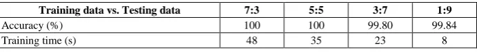
Table 2. Fault diagnosis results using TQWT and CNN
Training data vs. Testing data 7:3 5:5 3:7 1:9
Accuracy (%) 100 100 99.80 99.84
Training time (s) 48 35 23 8
It can be seen that the fault diagnosis accuracy of the proposed method based on TQWT and CNN is high for all the four ratios of training data against testing data. The fault diagnosis accuracies reach 100% for the ratios of 7:3 and 5:5, while the accuracies reach 99.8% for the ratios of 3:7 and 1:9. The training times of the four ratios are from 8 seconds to 48 seconds. When the ratio of training data to testing data is 1:9, the least training time (8 seconds) is needed and the fault diagnosis accuracy is still more than 99.8%, which verifies that the training procedure of the proposed method is very effective and efficient.
Fig. 7. Fault diagnosis accuracies for various motor operating conditions
Model generalization ability: In order to evaluate the generalization ability of the proposed algorithm, four other motor working conditions associated with the drive end bearing are used. The corresponding information about motor working status is listed in Table 3.
Table 3. Drive end bearing working condition data
Fault type Sample type
Number of samples Fault depth /mm Rotating speed r·min-1
Normal 100 -- 1750
Ball 100 0.14 1730
Inner ring 100 0.21 1730
Outer ring 100 0.07 1797
The experimental results indicate that fault diagnosis accuracies reach 100% when the ratios of training data against testing data is 7:3, 5:5, and 3:7; when the data ratio is 1:9, the accuracy can reach 97.78%. Therefore, the proposed algorithm has signifi-cant generalization ability.
The effect of TQWT: In order to verify the effect of TQWT denoising used in this research, the fault diagnosis accuracy using TQWT and CNN is compared with the results by directly using CNN on the original vibration data. The experimental results are given in Table 4.
Table 4. Comparison of the diagnosis accuracy by using CNN and TQWT+CNN
Sample proportion
7:3 5:5 3:7 1:9
Diagnostic method
Accuracy
(%) Loss
Accuracy
(%) Loss
Accuracy
(%) Loss
Accuracy
The results indicate that the fault diagnosis accuracy using TQWT+CNN is higher than the accuracy by using CNN without TQWT when the ratios of training data against testing data is 5:5, 3:7, and 1:9. In particular, accuracy is enhanced by about 3% for data ratio 1:9, which verifies that TQWT denoising is more effective for small training data sets.
Comparison with other method: The fault diagnosis accuracy of the proposed approach is compared with results reported in paper [32], which using wavelet trans-form and support vector machine to classify five operating conditions. Using 590 data sets for training and 145 data sets for testing, paper [32] obtain an optimal diagnosis result at 99.29%. Using the data and our algorithm based on TQWT and CNN, the fault diagnosis accuracy can reach 100%.
4
Conclusion
In this paper, a fault diagnosis method based on TQWT and CNN has been pro-posed and evaluated using the vibration data sets of seven motor operating conditions released by the Case Western Reserve University Bearing Data Center. The experi-mental results show:
The fault diagnosis accuracies of the presented method reach 100% when the ratios of training data against testing data are 7:3 and 5:5, while the accuracies reach 99.8for the ratios of 3:7 and 1:9
The training procedure of the proposed method is very effective and efficient, since when the ratio of training data to testing data is 1:9, only 8 seconds are needed for training
The proposed algorithm has good generalization ability, and its fault diagnosis accuracy is higher than reported accuracy using wavelets and support vector ma-chines.
5
Acknowledgement
This work was supported by the Natural Science Foundation of Hebei Province, China (Grant No. F2016502104), the Scientific Research Foundation for the Returned Overseas Chinese Scholars by The Ministry of Education of the People's Republic of China, and the Fundamental Research Funds for the Central Universities of China. The authors would like to thank Prof. Neil Bergmann for his kind support.
6
References
[2]Mekhilef S. Numerical and experimental analysis of vibratory signals for rolling bearing fault diagnosis. Mechanics, 2016, 22(3): 217-224. https://doi.org/10.57 55/j01.mech.22.3.11962
[3]Inturi V, Sabareesh G R, Supradeepan K, et al. Integrated condition monitoring scheme for bearing fault diagnosis of a wind turbine gearbox. Journal of Vibration and Control, 2019, 25(12): 1852-1865. https://doi.org/10.1177/1077546319841495
[4]Abdelkader R, Kaddour A, Derouiche Z. Enhancement of rolling bearing fault diagnosis based on improvement of empirical mode decomposition denoising method[J]. The Inter-national Journal of Advanced Manufacturing Technology, 2018, 97(5-8): 3099-3117. https ://doi.org/10.1007/s00170-018-2167-7
[5]Islam M MM, Kim J, Khan S A, et al. Reliable bearing fault diagnosis using Bayesian in-ference-based multi-class support vector machines. The Journal of the Acoustical Society of America, 2017, 141(2): EL89-EL95. https://doi.org/10.1121/1.4976038
[6]Tiwari R, Gupta V K, Kankar P K. Bearing fault diagnosis based on multi-scale permuta-tion entropy and adaptive neuro fuzzy classifier. Journal of Vibration and Control, 2015, 21(3): 461-467. https://doi.org/10.1177/1077546313490778
[7]Hinton G E, Salakhutdinov R R. Reducing the dimensionality of data with neural net-works. Science, 2006, 313(5786): 504-507. https://doi.org/10.1126/science.1127647
[8]Tang F, Mao B, Fadlullah Z M, et al. On a novel deep-learning-based intelligent partially overlapping channel assignment in SDN-IoT. IEEE Communications Magazine, 2018, 56(9): 80-86. https://doi.org/10.1109/mcom.2018.1701227
[9]Druzhkov P N, Kustikova V D. A survey of deep learning methods and software tools for image classification and object detection. Pattern Recognition and Image Analysis, 2016, 26(1): 9-15. https://doi.org/10.1134/s1054661816010065
[10]Sarikaya R, Hinton G E, Deoras A. Application of deep belief networks for natural lan-guage understanding. IEEE/ACM Transactions on Audio, Speech and Language Pro-cessing (TASLP), 2014, 22(4): 778-784. https://doi.org/10.1109/taslp.2014.2303296
[11]Xu F, Tse P W. Combined deep belief network in deep learning with affinity propagation clustering algorithm for roller bearings fault diagnosis without data label. Journal of Vi-bration and Control, 2019, 25(2): 473-482. https://doi.org/10.1177/1077546318783886
[12]Sohaib M, Kim C H, Kim J M. A hybrid feature model and deep-learning-based bearing fault diagnosis. Sensors, 2017, 17(12): 2876. https://doi.org/10.3390/s17122876
[13]Sun J, Yan C, Wen J. Intelligent bearing fault diagnosis method combining compressed da-ta acquisition and deep learning. IEEE Transactions on Instrumentation and Measurement, 2017, 67(1): 185-195. https://doi.org/10.1109/tim.2017.2759418
[14]LeCun Y, Bottou L, Bengio Y, et al. Gradient-based learning applied to document recogni-tion. Proceedings of the IEEE, 1998, 86(11): 2278-2324. https://doi.org/10.1109/5.726791
[15]Verstraete D, Ferrada A, Droguett E L, et al. Deep learning enabled fault diagnosis using time-frequency image analysis of rolling element bearings. Shock and Vibration, 2017, 2017. https://doi.org/10.1155/2017/5067651
[16]Eren L, Ince T, Kiranyaz S. A Generic Intelligent Bearing Fault Diagnosis System Using Compact Adaptive 1D CNN Classifier. Journal of Signal Processing Systems, 2019, 91(2): 179-189. https://doi.org/10.1007/s11265-018-1378-3
[17]Islam M. M. M., Kim J M. Automated bearing fault diagnosis scheme using 2D represen-tation of wavelet packet transform and deep convolutional neural network. Computers in Industry, 2019, 106: 142-153. https://doi.org/10.1016/j.compind.2019.01.008
trans-form. Computers in Industry, 106 (2019), p 48-59, 2019. https://doi.org/10.101 6/j.compind.2018.11.003
[19]R. Bendjillali, M. Beladgham, K. Merit, A. Taleb-Ahmed. Improved facial expression recognition based on DWT feature for deep CNN. Electronics, 2019, 3, 423.
https://doi.org/10.3390/electronics8030324
[20]H. Kutlu, E. Avc. A novel method for classifying liver and brain tumors using convolu-tional neural networks, discrete wavelet transform and long short-term memory networks. Sensors, 2019, 19, 1992. https://doi.org/10.3390/s19091992
[21]M. Guo, X. Zeng, D. Chen, N. Yang. Deep-learning-based earth fault detection using con-tinuous wavelet transform and convolutional neural network in resonant grounding distri-bution Systems. IEEE Sensors Journal, 2018, 18 (3): 1291-1299. https://doi.org/10.11 09/jsen.2017.2776238
[22]H. Liu, X. Mi, Y. Li. Smart deep learning based wind speed prediction model using wave-let packet decomposition, convolutional neural network and convolutional long short term memory network. Energy Conversion and Management, 166 (2018), pp. 120-131. https:// doi.org/10.1016/j.enconman.2018.04.021
[23]Selesnick I W. Wavelet transform with tunable Q-factor. IEEE transactions on signal pro-cessing, 2011, 59(8): 3560-3575. https://doi.org/10.1109/tsp.2011.2143711
[24]H. Wang; J. Chen, G. Dong. “Feature extraction of rolling bearing's early weak fault based on EEMD and tunable Q-factor wavelet transform,” Mechanical Systems and Signal Pro-cessing, vol. 48, no.1-2, pp. 103-119, 2014. https://doi.org/10.1016/j.ymssp.2014.04.006
[25]Cai G, Chen X, He Z. Sparsity-enabled signal decomposition using tunable Q-factor wave-let transform for fault feature extraction of gearbox. Mechanical Systems and Signal Pro-cessing, 2013, 41(1-2): 34-53. https://doi.org/10.1016/j.ymssp.2013.06.035
[26]Selesnick I W. Resonance-based signal decomposition: A new sparsity-enabled signal analysis method. Signal Processing, 2011, 91(12): 2793-2809. https://doi.org/10.101 6/j.sigpro.2010.10.018
[27]Case Western Reserve University Bearing Data Center Website [DB/OL]. [2019-08-03]. http://csegroups.case.edu/bearingdatacenter/home.
[28]Ma P, Zhang H, Fan W, et al. Early fault diagnosis of bearing based on frequency band ex-traction and improved tunable Q-factor wavelet transform. Measurement, 2019, 137: 189-202. https://doi.org/10.1016/j.measurement.2019.01.036
[29]Bharath I, Devendiran S, Mathew A T. Bearing Condition Monitoring Using Tunable Q-Factor Wavelet Transform, Spectral Features and Classification Algorithm. Materials To-day: Proceedings, 2018, 5(5): 11476-11490. https://doi.org/10.1016/j.matpr.2018.02.115
[30]Zhao Z, Chen X, Ding B, et al. TQWT-based multi-scale dictionary learning for rotating machinery fault diagnosis. 2017 13th IEEE Conference on Automation Science and Engi-neering (CASE). IEEE, 2017: 554-559. https://doi.org/10.1109/coase.2017.8256162
[31]Shi J, Liang M. Intelligent bearing fault signature extraction via iterative oscillatory behav-ior based signal decomposition (IOBSD). Expert Systems with Applications, 2016, 45:
40-55. https://doi.org/10.1016/j.eswa.2015.09.039
7
Authors
Liqun Hou (corresponding author) is an Associate Professor in the School of Con-trol and Computer Engineering, North China Electric Power University, Baoding 071003, China. E-mail: [email protected].
Zijing Li is with the School of Control and Computer Engineering, North China Electric Power University, Baoding 071003, China. E-mail: [email protected].