Comparison of GPR Random Noise Attenuation Using Autoregressive FX Method and Tunable Quality Factor Wavelet Transform TQWT with Soft and Hard Thresholding

(1)

ISSN Online: 2159-4481 ISSN Print: 2159-4465

DOI: 10.4236/jsip.2019.101003 Dec. 29, 2018 19 Journal of Signal and Information Processing

Comparison of GPR Random Noise Attenuation

Using Autoregressive-FX Method and Tunable

Quality Factor Wavelet Transform TQWT with

Soft and Hard Thresholding

Amin Ebrahimib Bardar

1

_{, Behrooz Oskooi}

1*

_{, Alireza Goudarzi}

2

1_{Institute of Geophysics, University of Tehran, Tehran, Iran}

2_{Faculty of Sciences and Modern Technologies, Graduate University of Advanced Technology, Kerman, Iran}

Abstract

Ground Penetration Radar is a controlled source geophysical method which uses high frequency electromagnetic waves to study shallow layers. Resolu-tion of this method depends on difference of electrical properties between target and surrounding electrical medium, target geometry and used band-width. The wavelet transform is used extensively in signal analysis and noise attenuation. In addition, wavelet domain allows local precise descriptions of signal behavior. The Fourier coefficient represents a component for all time and therefore local events must be described by the phase characteristic which can be abolished or strengthened over a large period of time. Finally basis of Auto Regression (AR) is the fitting of an appropriate model on data, which in practice results in more information from data process. Estimation of the pa-rameters of the regression model (AR) is very important. In order to obtain a higher-resolution spectral estimation than other models, recursive operator is a suitable tool. Generally, it is much easier to work with an Auto Regression model. Results shows that the TQWT in soft thresholding mode can attenuate random noise far better than TQWT in hard thresholding mode and Autore-gressive-FX method.

Keywords

GPR, Autoregressive-FX, Tunable Quality Factor Wavelet Transform TQWT

1. Introduction

Ground Penetration Radar is a controlled source geophysical method which uses How to cite this paper: Bardar, A.E.,

Oskooi, B. and Goudarzi, A. (2019) Com-parison of GPR Random Noise Attenuation Using Autoregressive-FX Method and Tunable Quality Factor Wavelet Transform TQWT with Soft and Hard Thresholding. Journal of Signal and Information Processing, 10, 19-35.

https://doi.org/10.4236/jsip.2019.101003

Received: April 17, 2018 Accepted: December 26, 2018 Published: December 29, 2018

http://creativecommons.org/licenses/by/4.0/

(2)

DOI: 10.4236/jsip.2019.101003 20 Journal of Signal and Information Processing

high frequency electromagnetic waves to study shallow layers. The use of this method began in 1956 and has been developed since the 1970s. GPR system has been commercially available since the 1980s, and has been widely used since the mid-decade. In the GPR method, high frequency electromagnetic waves (from 12.5 to 2300 MHz) transmit to the earth and these waves are reflected by objects or clear boundaries between the underground layers. Electromagnetic reflections are created by the difference in electrical conductivity (dielectric constant) be-tween materials that pass electromagnetic waves. GPR electromagnetic waves pass through materials that are electrically conductive, but they are heavily ab-sorbed when passing through high-conductivity materials such as clays, organic acid soils and saturated saline water [1].

Resolution of GPR varies from depth of centimeters to a several meters with maximum depth of about 100 meters. Resolution of this method depends on difference of electrical properties between target and surrounding electrical me-dium, target geometry and used bandwidth. Resolution of this method can be high which can recognized fine layers in near surface structures and objects in the ground can be well [2].

The wavelet transform is used extensively in signal analysis and noise attenua-tion. In addition, wavelet domain allows local precise descriptions of signal be-havior. The Fourier coefficient represents a component for all time and therefore local events must be described by the phase characteristic which can be ab-olished or strengthened over a large period of time. Wavelet expansion coeffi-cients represents a component which is local itself and convenient for interpre-tation. The wavelet Transform may allow separation of signal components which overlaps in time and frequency. Wavelets can be designed to fit the unique ap-plications because they are also customizable and tunable and there is not just one wavelet. They are ideal for adaptive devices that adjust themselves to the signal. Finally, production of wavelets and the calculation of discrete wavelet transforms (DWT) are well suited to digital computing [3].

Finally basis of Auto Regression (AR) is the fitting of an appropriate model on data, which in practice results in more information from data process. Estima-tion of the parameters of the regression model (AR) is very important. Also use of a suitable model is very important in approximation of random signals spec-trum, especially in parametric methods. Parametric methods of power spectrum estimation are based on selecting the appropriate model for the data [4].

In order to obtain a higher-resolution spectral estimation than other models, recursive operator is a suitable tool. Generally, it is much easier to work with an Auto Regression model. For this reason, suitable techniques are presented for estimating of model parameters [5].

2. Problem Definition and Research Method

(3)

( )

( ) ( )

X t =S t ∗ω y +n t (1)

In Equation (1), the earth reflection series s(t) is matched in the wavelet due to the spring w(t) and the noise n(t) is added to the data, which must be corrected. Since it is impossible to eliminate all of the noise, then the denoising is done with the aim of obtaining X(t) is as close as possible to s(t) [6].

In this research, noise attenuation method of auto regressive on wavelet and f-x domains was used to reduce the noise of the GPR signal. First AR operator and definition of f-x domain will illustrate and explained using some examples. Ultimately, all methods will be applied to real and synthetic data of the GPR signal and their results will be compared together.

3. Wavelet Transform with Tunable Quality Factor (TQWT)

In this section, a wavelet transform method is described where it easily uses the Q factor and wavelet transform process can be controlled using the periodic na-ture of the signal. The function of scale has real values. The Q factor is a ratio of the frequency center to signal bandwidth. Most wavelet transform methods have a poor ability to control behavior of signal frequencies. The TQWT method is completely discrete, it has a complete signal reconstruction ability and mean re-dundancy.

3.1. Low Pass Scale

The low-frequency region of the signal is analyzed using the low-pass function. If the scale parameter α is chosen for the low-pass scale function part, the sampling changes to αfs, where fs is sampling frequency of the input signal.

If 0< ≤

α

1_{, then the function of the low-pass signal changes:}

( )

, π

Y ω =X αω ω ≤ (2)

And if, low pass function changes a signal like:

( )

, π

0, π π

X

Y ω αω ω α

α ω

 ≤

 = 

< <

 (3)

Note that low-pass function keeps signal behavior around a zero frequency according to Figure 1.

3.2. High Pass Scale

The high-frequency signal region is analyzed by high-frequency scale function. If the scale parameter β _{is selected for the high-pass section function, the} sam-pling is changed to βfs, which fs is sampling frequency of input signal. If

0< ≤β 1, the of the high-pass scale function will change such a signal:

( )

(

)

(

)

(

)

1 π , 0 π

1 π , π π

X Y

X

βω β ω

ω

βω β ω

 + − < <

 = 

− − − < <

 (4)

(4)

[image:4.595.262.485.71.536.2]

Figure 1. Low-pass function keeps signal behavior around the

zero frequency [7]. (a) Low-pass scaling block diagram; (b) low-pass scaling with α < 1; (c) low-pass scaling with α > 1.

( )

(

)

(

)

(

)

(

)

(

)

(

)

(

)

0, 1 1 π

1 π , 1 1 π π

1 π , π 1 1 π

Y X

X

ω β

ω βω β β ω

βω β ω β

 _{< −}



= + − − < <



− − − < < − 

(5)

The high-pass scale function keeps signal around the Nyquist frequency ac-cording to Figure 2.

(5)

Using a frequent dual channel filter, the TQWT method is applied. This transform is represented by three steps in Figure 3 [7].

( )j

_{( )}

_n

ω

_{denotes the subband in}_j_{th step and it’s generated for}_j_{= 1 high-pass} subband in the first stage. The subband bandwidth of the jth frequency is

1 _.

j s

f

α − _Also s

f is a sampling frequency of input data.

Figure 4 shows frequency response H1j

( )

ω

for 1≤ ≤j J for 4 values of

[image:5.595.259.488.204.687.2]

(

β α,

)

. By changing these variables, spectral frequency decomposition can be controlled.

Figure 2. The high-pass scale function keeps signal around the

(6)

[image:6.595.233.512.76.155.2]

Figure 3. Using a frequent dual channel filter, the TQWT method is

ap-plied. This transform is represented by three steps in figure [7].

Figure 4. Frequency response H_1^j (ω) for 1 ≤ j ≤ J for 4 values of (β, α) [7].

3.3. Redundancy

The dual-channel filter in Figure 3 with the factor α β+ _{is redundant. If this}

filter is repeated in the low-pass, the Redundancy factor is:

1

r β

α

=

− (6)

This relation is deduced from the fact that a sampling frequency under the jth subband for j≥1_{is determined by} j 1

s

f

βα − _{, So sampling frequency is}

equiva-lent to (6).

3.4. Central Frequency

The frequency response in the jth step H1j

( )

ω

is nonzero at the distance

[image:6.595.213.535.195.498.2]

(7)

(

)

1 1

1 1 j π, 2 j π,

ω

_{= −}

β α

−

ω

₌

α

− ₍₇₎

The central frequency of the jth stage is approximately average

(

ω ω1, 2

)

.

(

)

0 1₂ 1 2 j2₂ π

β

ω ω ω α

α

−

= + = ₍₈₎

This relationship is based on the sampling frequency: 2

4 j

c s

f α β f

α

−

= ₍₉₎

The bandwidth of the frequency response under the jth subband is about a half of bandwidths of all frequencies that have a non-zero response.

(

)

1

1 2

1 1 _π

2 2

j

BW ₌ ω ω₋ ₌ βα − ₍₁₀₎

If the Q factor is expressed on the basis of α β,

2 : c Q BW

ω

β

−

= = (11)

Note that Q is not dependent on the stage. A Transform method is Q constant and depends only on filter bank parameters. To determine α and β, they are re-written based on r and Q:

2 , 1

1

Q r

β

β = α = −

+ (12)

A Q factor must be greater or equal to 1, and if Q is equal to 1, wavelet trans-form builds a second derivative of a Gaussian function. If Q is greater than one that means signal has a higher periodic behavior and the Oversampling rate should be greater than one. If r is near 1, the transition region is very thin and the time response of the wavelet is not properly determined. If r≈1 makes a sinc wavelet, then it’s therefore optimal to r≥3_.

When the signal is staircase oscillatory, a number of vanishing moments of the wavelet transform is considered. This is not the case when we talk about a periodic signal like a GPR signal. The number of steps for this type of wavelet transform is limited by the length of the signal. After a certain stage, the signal will be very short to become two samples. If countless steps are taken, conver-sion of these steps is difficult to reconstruct. J must be determined so that the wavelet does not extend beyond the length of the category.

max log 8 1 log N J β α       _ _   =        _{ }    (13)

4. F-X Domain

(8)

extracted in terms of frequency [8].

( )

2

1 _d

2π

E=

_∫

_+∞−∞ x f f (14)

Given that in time domain, input data or signal, for each frequency is shown as sinusoidal functions in the location, the separation of the signal from the noise is made easier. Therefore, we will investigate predictive filter in this do-main. This method assumes that a class is composed of delayed impacts in ac-cordance with Figure 5.

The f-x prediction filter method is very useful method to attenuate random noise. 1. Selesnick, (I.W. Sparse signal representations using the tunable Q-factor wavelet transform. in Wavelets and Sparsity XIV. 2011. International Society for Optics and Photonics.)

In this method, it is assumed that trends are linear. The seismic section can be divided into smaller windows in cases where trends are not linear, in order to sa-tisfy the assumption given that trends in that window are linear. Assume that a seismic U x t

( )

, is a sequence of impacts with different domains defined as [9]:

( )

(

( )

)

1

, N j j

j

U x t A t g xδ

=

∑

− ₍₁₅₎

where t is the time, x is the lateral position, Ai is the jth impact, and g xj

( )

is the delay function that represents the event’s form. Considering Fourier trans-form of (15) we have:

(

)

( )

1

, N e i g xj

j j

U xω A −ω

=

∑

₍₁₆₎

Since exponential functions can be written as a set of sinuses and cosines, in (16), the hypothesized seismic traces are converted into a set of sinuses and co-sines as functions of ω and x. Since the f-x filter only predicts linear data, events should be linear to x. So the function g xj

( )

must be linear [9]. Given the li-nearity of g x U xj

( ) (

⋅ ,ω

)

in the frequency domain, (16) will be:

(

)

1

, N e i b xj

j j

U xω C −ω

=

[image:8.595.273.481.517.707.2]

=

∑

₍₁₇₎

(9)

DOI: 10.4236/jsip.2019.101003 27 Journal of Signal and Information Processing j

C is a conjugate constant, which depends on the source power and the ref-lection coefficient, and Bj is the gradient of the linear event. (17) Shows that by linearization assuming, the function U x

(

,ω

)

is completely sinusoidally in x, which means that this function is predictable and predictable. Therefore, the signal is a complex exponential function in terms of x in the time-frequency domain and it will be predictable [10]. The Wiener filter is an optimal stable li-near filter for noise-damaged images. The Wiener filter needs to assume that the signal and noise are secondarily stable. For this purpose, noises are considered frames with a mean zero. The procedure used in this method is to minimize the sum of squares of the difference between output signal and the actual output signal from the filter. The Wiener filter is incapable of reconstructing the fre-quency components that are damaged by noise, and can only eliminate them. This filter is incapable of neutralizing the image of the image and has a low ve-locity. To speed up this filter, we can use this filter to obtain a shock response, reversed the fast Fourier transform [11]. To speed up this filter, we can use in-verse fast Fourier transform and obtain the impulse response.

5. Autoregressive Vector

Classical models of time series are divided into stationary and non-stationary sections. Autoregressive vector is part of classic static time series model that we will discuss in this article. One of the limitations of our models is that they im-pose a one-way relationship whose predictor variables are influenced by pre-dicted variables which this process must be reversed. However, in many cases, the reversal of this action must also be made where the variables affect each oth-er. In this framework, all variables behave symmetrically [12]. In an Autoregres-sive model, the variables are predicted using a linear combination of the pre-vious values of the variables. The term Autoregressive represents a regression of the variable against itself [13]. The regression model is defined as follows:

1 1

t t p t p t

y = +c a y₋ + +_ a y₋ +ε ₍₁₈₎ where c is constant and εt is a white noise with mean zero and the variables

2 ε

σ and ai are the parameters of the model. In this case, yt is called the p-th

Autoregressive model with and is represented by AR (p). An Autoregressive structure is simple, useful, and easy to understand in a wide range of fields. The first-order Autoregressive is defined as follows [13].

1 1

t t t

y =a y− +ε (19) Assumptions:

Firstly, the residue is expected to be zero

,

0 with

1,2

i t

E

  =

_{ }

ε

i

=

₍₂₀₎

And secondly, errors are not self-correlated.

, , 0 with

i t j

E

ε ε

τ = t≠

τ

(21)

(10)

range of different time series. Figure 6 shows main steps of Autoregressive vec-tor.

Autoregressive models do not allow us to explain on causal relationships. This is especially applies when Autoregressive models are merely generalized for the processing of unknown time series. While a causal interpretation requires a basic cost model. However Autoregression provides a proper interpretation of the va-riables shown [5].

In order to increase the signal-to-noise ratio of a multi-point signal (S/N), firstly the Autoregression vector of the noisy data is estimated and shown as a

ˆ_j

A . Then, the forward estimated of denoised data is obtained by the following equation [14].

1

ˆ

ˆf M , 1, ,

k j k j

j

g A g − k M N

=

∑

= + _ ₍₂₂₎

Similarly, the estimated inverse equation of de-noised data are obtained:

* 1

ˆ

ˆb M , 1, ,

k j k j

j

g A g + k M N M

=

∑

= + _ − ₍₂₃₎

*

ˆ_j

A represents the complex conjugate of Autoregressive vector operator. The final equation of the de-noised data are obtained by mean for forward and in-verse estimates:

ˆ ˆ

ˆ

2

f b

t k k

k g g

[image:10.595.222.531.374.708.2]

g = + ₍₂₄₎

(11)

6. Applying Autoregressive Filter in f-x and Tunable Quality

Wavelet Transform (TQWT) Domain on GPR Data

Given that the purpose here is to reduce the random noise, in the first step a random noise should be added to the section which obtained from synthetic models. For synthetic data generation, the ground model is firstly considered with arbitrary coefficients. Given the similarity in wave propagation of electro-magnetic waves and seismic waves, synthetic modeling of GPR and seismic data are analogous. Random noise is added to synthetic model and various de-noising methods which presented in this article apply to it. After denoising of synthetic model, real GPR data will be denoised. Here, by applying linear Autoregression modeling on wavelet and f-x domain, random noise in actual data will be wea-kened. The procedure is applying these steps on real data in wavelet domain and then transforms the denoised data waveform from wavelet domain. After these steps and in next section, results will be compared and evaluated.

6.1. Wavelet Function of Synthetic Data Generator

The wavelet used to generate this synthetic data is the Ricker Wavelet. This wavelet is formulated as [15]:

( )

_t

(

₁ _π2 2 2_{f t}

) (

_exp _π2 2 2_{f t}

)

ω = − − (25)

( )

t

ω is Ricker wavelet, t is time and f is the central frequency. Ricker wavelet is symmetric in time domain and has zero mean (

_∫

_−∞+∞r

( )

τ τd =0_).

The generated synthetic signal is formulated as:

( )

X t =S t ∗ω t +n t (26)

In (26), S t

( )

is a received that is correlated with the Ricker wavelet (as a synthetic wavelet source). n t

( )

is a random noise that is added to the input signal.

6.2. Synthetic Model Denoising

6.2.1. TQWT Denoising in Soft and Hard Thresholding

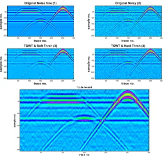
To evaluate efficiency of mentioned denoising methods, an artificial section considered which is consisting of five layers and three pipes according to Figure 7. Based on that section, GPR data will be generated as Figure 8-1 and random noise will be added according to Figure 8-2. The sampling frequency is 40 ns and the noise is the 40 dB white Gaussian noise. As shown in Figure 8-2, the path of the layers are somewhat lost particularly thinner layers. Also, the promi-nence and boundary of layers and pipes throughout the noisy cross-section have been damaged.

Figure 8-1 shows the GPR cross section in the time domain and in Figure 8-2

(12)

in noise attenuation and that noises are still present.

[image:12.595.235.513.220.322.2]

The only difference between noisy and the hard thresholding denoised signals are in a deformation of the noises. The noises are somewhat diminished, but it shows another form of noise as an elongation along the axis of time. The boun-daries of layers and hyperbolas are still confusing and effect of noise is not dimi-nished. Figure 8-3 shows application of the TQWT with a soft thresholding method. This method has been far more successful in noise attenuation. A sig-nificant part of the noise has been attenuated, and boundaries of layers and hyperbolas are significantly clear.

Figure 7. Synthetic model which consists of five layers and two shapes of a

pipe and a duct. Their conductivity and dielectric constant are shown.

Figure 8. 1—Synthetic data, 2—Synthetic data with white noise, 3—Denoised data by soft

thresholding TQWT, 4—Denoised data by Hard Thresholding TQWT, 5—Denoised by Autoregressive-FX.

A

B

C

D

E

P P

A=(εr=1,σ=0mS/m), B(=εr=9,σ=1mS/m), C=(εr=25,σ=5mS/m),

D=(εr=9,σ=1mS/m), E=(εr=25,σ=5mS/m), P=(εr=16,σ=1mS/m)

P

Original Noise free (1)

trace no.

sa

m

ple

no.

50 100 150 200 250 300

50

100

150

200

250

Original Noisy (2)

trace no.

sa

m

ple

no.

50 100 150 200 250 300

50

100

150

200

250

TQWT & Soft Thrsh (3)

trace no.

sa

m

ple

no.

50 100 150 200 250 300

50

100

150

200

250

TQWT & Hard Thrsh (4)

trace no.

sa

m

ple

no.

50 100 150 200 250 300

50 100 150 200 250 f-x denoised trace no. sa m ple no.

50 100 150 200 250 300

50

100

150

200

[image:12.595.211.537.367.683.2]

(13)

High-frequency noises have been far more attenuated, but the elongation por-tion is also included in this filter. But this elongapor-tion is significantly less than the hard thresholding. Therefore, signal is significantly improved by soft threshold-ing method compared to the hard thresholdthreshold-ing.

6.2.2. Investigation of TQWT Power Spectrum Results in Soft and Hard Thresholds

Figure 9 shows the results of the power spectrum. Soft thresholding power spectrum results (blue) at low to moderate frequencies are the most reduced in comparison to the power spectrum of input data (red). Its reduction compared to the hard thresholding (black) is remarkable. The gradient of soft thresholding power spectrum is also confirmed with the power spectrum of signal which in-dicates the sustaining of signal in this method. The highest level of noise attenu-ation in soft thresholding was also achieved with random noise at high frequen-cies. But the point is that after a certain frequency (2.10 MHz) and at high fre-quencies, noise gain is quite clear in both the soft and hard thresholding.

6.2.3. Autoregressive-FX Filter

To denoising in this section, Autoregressive filtering is applied in time domain.

Figure 8-5 shows data after denoising by Autoregressive model in the time do-main. After applying the Autoregressive filter is time domain, it is observed that the noise has been attenuated and the boundaries of the layers are specified much well. In Figure 8-5 after applying the Autoregressive filter, layer bounda-ries are well detectable, softened, and the noise is well reduced. The point is elongation in direction of axis of time is happening due to the application of the filter. But in general, it has successfully restored the boundary between layers and parabolas.

7. Real Data Denoising

In this section the filtering on real data will be discussed. Firstly the Autoregres-sive-FX filter and after that the TQWT in soft and hard thresholding ways.

7.1. Autoregressive-FX Filter

With respect to Figure 10, it can be concluded that the AR filter has been rela-tively successful in noise attenuation. Layer and hyperbolic boundaries have been improved and some of the high-frequency noise has been eliminated. It can be said that the signal is denoised, but some of the high-frequency noise is still dominant. As we said before, our noise is random does not have a definite origin. In Figure 10, we see that the right side contains a lot of noise, especially at high arrivals and in most parts of the data it is completely polluted by noise which that part of the traces are covered.

7.2. Real Data Noise Attenuation Using TQWT

(14)

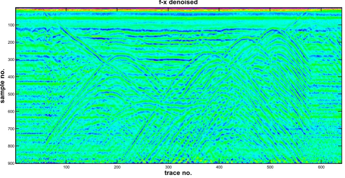
[image:14.595.183.537.277.454.2]

and Figure 11-3, it is observed that in hard thresholding method, significant amounts of high-frequency noise are observed. Also, the high-gain times are to-tally infected with high-frequency noise and no noise reduction has been made. Also high arrivals in traces are completely infected with high-frequency noise and noise attenuation is not successful. But the soft thresholding completely at-tenuated the noise and like raw synthetic data, the Background is completely out of high-frequency noise. Of course, part of the elongations marks still shows up, but the boundary of the deep layers is well recovered. Reflection of the hyperbo-las and their interference points are clear and none of them have been removed. So that it can be said that the noise in this section of the signal is completely eliminated and the noise attenuation is very well done. This results are con-firmed by power spectrum of real data by TQWT hard and soft thresholding in

[image:14.595.186.537.525.706.2]

Figure 12.

Figure 9. Power spectrum in terms of synthetic data frequency. 1—Red: raw input signal.

2—Black: Input noisy data. 3—Blue: Denoised output data using soft thresholding TQWT. 4—Green: Output data denoised by TQWT Hard Thresholding. 5—Dashed Brown: Denoised synthetic data using Autoregressive-FX filter.

Figure 10. Real data noise attenuation using Autoregressive-FX.

105 106

10-3 10-2 10-1 100 101

Frequency(Hz)

P

o

we

r

f-x denoised

trace no.

sa

m

ple

no.

100 200 300 400 500 600

(15)

[image:15.595.181.536.73.376.2]

Figure 11. 1—Real data, 2—Denoised by soft thresholding TQWT, 3—Denoised by Hard

thre-sholding TQWT.

Figure 12. Power spectrum of real data. 1—Red: Raw signal, 2—Black: Denoised by soft

thre-sholding TQWT, 3—Denoised by Hard threthre-sholding TQWT.

8. Conclusions

As stated several factors make the GPR data noisy such as mobile networks, power stations, etc. Considering that the increase of signal-to-noise ratio is the main objective of this research a method was chosen that to attenuating the noise and minimizes the damage to the signal. In this paper synthetic and real GPR data was denoised with the TQWT in two soft and hard thresholding and the Autoregressive-FX filter. According to the results, it can be concluded that the hard thresholding method is not suitable. Results do not show a good

im-Original (1)

trace no.

s

a

m

ple

no.

100 200 300 400 500 600

200

400

600

800

TQWT & Soft Thrsh (2)

trace no.

s

a

m

ple

no.

100 200 300 400 500 600

200

400

600

800

TQWT & Hard Thrsh (3)

trace no.

s

a

m

ple

no.

100 200 300 400 500 600

200

400

600

800

105

106

10-2 10-1

100

101

Frequency(Hz)

Po

we

r

Input noisy.

[image:15.595.184.536.414.556.2]

(16)

provement, especially at low frequencies, most of the noise remains, and the elongations which caused by hard threshold has also been added to these noises.

However, in the soft thresholding problem of elongation noise is observed. But a significant part of the noise is attenuated and high-frequency noise has been eliminated. After the deactivation, the spikes from the real signal are well observed. Also boundaries of layers and hyperbolas are also returned. The Au-toregressive-FX method has succeeded to denoising of high-frequency noise. The layer boundaries are also clear, but less denoising has been achieved com-pared to the soft thresholding TQWT. Also layer boundaries are less detected and part of high-frequency noise is still seen.

As a result, the wavelet domain provides a suitable frequency resolution for noise attenuation. But the type of filter applied to the wavelet transform also af-fects denoising. The TQWT method has a good frequency resolution because it operates in the wavelet domain, but the results of hard thresholding indicate that the selection of the appropriate filter for de-noising substantially changes results. Finally, by comparing all of results, it can be said that the TQWT soft sholding method has been much more successful compared to the hard thre-sholding and Autoregressive-FX in denoising and converting the actual signal.

Conflicts of Interest

The authors declare no conflicts of interest regarding the publication of this pa-per.

References

[1] Annan, A.P. (2001) Ground Penetrating Radar. Workshop Notes, September 2001, 192.

[2] Daniels, D.J. (2004) Ground Penetrating Radar. 734.

https://doi.org/10.1049/PBRA015E

[3] Burrus, S.C. and Gopinath, R.A. (2013) Wavelets and Wavelet Transforms. Rice University, Houston, 1-281.

[4] Kim, J.H. and Cho, S.J. (2007) Removal of Rining Noise in GPR Data by Signal Processing. Geosciences Journal, 11, 75-81. https://doi.org/10.1007/BF02910382

[5] Leonard, M. and Kennatt, B.L.N. (2008) Multicomponent Autoregressive Tech-niques for the Analysis of Seismograms. Physics of the Earth and Planetary Inte-riors, 113.

[6] Oskooi, B., Julayusefi, M. and Goudarzi, A. (2015) GPR Noise Reduction Based on Wavelet Thresholdings. Arabian Journal of Geosciences, 2937-2951.

https://doi.org/10.1007/s12517-014-1339-5

[7] Selesnick, I.W. (2011) Sparse Signal Representations Using the Tunable Q-Factor Wavelet Transform. Proc. SPIE 8138, Wavelets and Sparsity XIV, 81381U. [8] Yilmaz, O. (2000) Seismic Data Analysis: Processing, Inversion, and Interpretation

of Seismic Data. Society of Exploration Geophysicists, 1-7.

[9] Canales, L.L. (1984) Random Noise Reduction. 54th Ann. Mtg. Society of Explora-tion Geophysicists. https://doi.org/10.1190/1.1894168

(17)

DOI: 10.4236/jsip.2019.101003 35 Journal of Signal and Information Processing Thesis Present to Ryerson University.

[11] Harrison, M.P. f-x Linear Prediction Filtering of Seismic Images.

[12] Luetkepohl, H. (2011) Vector Autoregressive Models, Economics Departments, In-stitutes and Research Centers in the World.

https://ideas.repec.org/p/eui/euiwps/eco2011-30.html

[13] Fuss, R. (2007) Vector Autoregressive Models. Albert-Ludwigs-University of Frei-burg.

[14] Naghizadeh, M. and Sacchi, M. (2012) Multicomponent f-x Seismic Random Noise Attenuation via Vector Autoregressive Operators. Geophysics, 77, V91-V99. [15] Wang, Y. (2015) Frequencies of the Ricker Wavelet. Geophysics, A31-A37.