* Corresponding author Tel: +989166635625, E-mail address: [email protected] (F. Kolivand).
Determination of settlement trough width and optimization of soil
behavior parameters based on the design of experiment method (DOE)
Farshad Kolivand
a, *, Reza Rahmannejad
aa Mining Engineering Department, Faculty of Engineering, Shahid Bahonar University of Kerman, Kerman, Iran
ABSTRACT
The expansion of a settlement trough is an important factor in risk assessment of the tunneling induced settlement. The increase of settlement trough causes damages and requires buildings to be included in the impact zone. This paper conducts an estimation of the settlement trough width (STW) using empirical approaches, field measurement data, and numerical solutions. The credibility of the numerical results is affected by the accuracy of the input data such as geotechnical parameters (E, c, and φ). Therefore, an approach is used in which the 3D finite element modeling (FEM) and Taguchi’s experimental design are combined to estimate the geotechnical parameters (E, c, and φ). The field settlement measurements are used to validate the numerical modeling results. The results indicate that Taguchi’s (DOE) method is an effective approach to estimate the geotechnical parameters. In addition, the numerical modeling provides a wider settlement trough than the empirical methods and the instrumentation data. However, the maximum settlement in numerical modeling has the least deviation of the field settlement data. There is a good agreement between empirical approaches and field settlement data to estimate i-value and STW parameter. The results of numerical simulation overestimated the settlement trough width, which causes more buildings to be included in the tunnel impact zone. It demands more extensive study to assess the tunneling induced building damage, which is more conservative.
Keywords : Design of experiment (DOE), Geotechnical parameters, Point of inflection, Settlement trough width (STW), Taguchi’s method
1.
Introduction
Urban growth is continuously increasing, and is expected to reach 60% in 2030, and 70% in 2050 [1]. Expanding cities increase the demand for the development of the public transportation system such as subway tunnels. However, tunnel excavation causes surface settlement trough, which may affect the safety of the adjacent buildings. Therefore, tunneling designs require precision assessment of the settlement parameters such as the settlement trough width (STW) and the point of inflection (i). The width settlement trough determines the buildings included in the tunnel impact zone, and is an important factor in the risk assessment of the tunneling induced settlement.
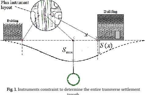
The proposed empirical approaches for predicting the surface settlement is based on Peck’s studies (1969) [2]. The transverse settlement trough is described commonly by the Gaussian function probability curve [2]. Many authors have proposed different relations to predict the STW parameter and the inflection point [2-14]. The increase of the surface settlement may cause more buildings to be damaged. The tunneling effect study on the safety of the buildings requires a proper understanding of the settlement trough width. As seen in Fig. 1, the instrument settlement data determines only a limited part of the transverse settlement curve. It is necessary to determine the entire extent of the settlement trough to study the damage assessment of the buildings (Fig. 1). The extension of the settlement curve under the buildings requires estimation of the STW parameter (dash line). Estimation of the STW parameter needs the determination of the inflection point parameter (i).
Fig. 1. Instruments constraint to determine the entire transverse settlement trough.
In this paper, the STW parameter is investigated by different approaches, including empirical solutions, field measurement data, and numerical modeling. In geotechnical systems, the accuracy of the geotechnical parameters is important, which influences the credibility of a numerical model. Therefore, an accurate estimation of the geotechnical parameters is vital for evaluation of the building-tunnel interaction.
Taguchi’s (DOE) principle was introduced by R. A. Fisher and later improved in the 1940s by Taguchi [15]. It is a statistical method to optimize the process factors and recuperate the quality of manufactured products. The application of DOE was developed to other fields such as environmental sciences [16-18], agricultural sciences [19], medical sciences [20-23], chemistry [24, 25], physics [26-28], statistics [29-32], management and business [33-35], optimization of the operating
Article History:
parameters [36, 37], marketing, advertising, etc. [38]. Taguchi’s DOE is used when there are many input parameters and it requires a simultaneous influence of these inputs on the output response [39, 40]. The aim of this research is to investigate the STW parameter by empirical solutions, field measurement data, and numerical modeling. Appropriate estimation of the geotechnical parameters is a key aspect of numerical modeling. First, the Taguchi’s DOE method is utilized for optimization of the modulus of elasticity (E), cohesion (c), and the internal friction angle (φ). Then, the optimum geotechnical parameters are applied to 3D numerical models to investigate the STW parameter. The numerical models are calibrated through comparison with field measurement data. The STW parameter is calculated based on the suggested empirical formula by different authors. Afterward, the derived settlement curves are plotted based on the STW’s values. The field measurement data is used to estimate the extension of the settlement trough and the inflection point. Finally, the results of numerical modeling, empirical approaches, and filed settlement data are compared.
2.
Location and ground conditions
2.1. Location
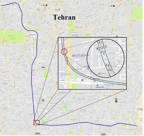
The east-west section of Tehran metro line No. 7 is designed to be 12 km long. The tunnel is excavated using an earth pressure balance (EPB) TBM manufactured by SELI Technology Corporation. The tunnel diameter is 9.14 m, which lines by segment thickness 0.35m. A plan of the tunnel route and section under study is illustrated in Fig. 2.
Fig. 2. The tunnel route line No. 7 and section under study, Tehran Metro, Iran.
2.2. Ground conditions
Tehran plain mainly consists of alluvial materials, which is classified into four formations identified as A, B (Bn and Bs), C, and D by Rieben (1955 & 1966) and Pedrami (1981) [41, 42]. The underlays of the tunnel route consist of a series of alluvial layers with different grain size distribution (from clay to boulder) [43]. The stratigraphy of Tehran Alluvium formations and geotechnical properties of soil layers is illustrated in Fig. 3. The detailed geotechnical investigations are performed by excavation of 61 boreholes (a total length of 2487.7 m) and 16 test pits (a total length of 296.95 m). These investigations mainly included some field tests and surveying, laboratory tests, and desk studies. The field tests include plate loading test (PLT), in-situ shear test,
pressuremeter test, standard penetration test(SPT), Lufran permeability test, and in-situ density test. The laboratory tests comprise the direct shear test, triaxial test, particle size analysis, Atterberg limits test, consolidation, permeability, Los Angeles Abrasion test, and X-ray fluorescence (XRF). The desk studies include the collection of the existing data such as previous reports, in-situ test results, and data processing and analyzing [44].
(a)
(b)
Fig. 3. a) The stratigraphy of Tehran Alluvium formations. b) Geological and geometrical properties of soil layers.
3.
Field measurement data
The field measurements for tunneling in an urban area aim to: a) Assessment and refining the design;
b) Improving the excavation operation and the tunneling modes; and c) Minimizing the surface settlements due to the deformations induced by the tunnel excavation. These supervisory data can be used to control the behavior of the adjacent buildings both qualitatively and quantitatively.
(1 to 3 pins per cross section). The settlement pins basically consist of a steel rod, which applied as the benchmark. The leveling operation is conducted by high-precision cameras. The installed instrumentation layout in the section under study is illustrated in Fig. 2. The field measured settlements are compared to calculated settlements to validate the numerical modeling results. The field settlement measurements of the section under study (Settlement points C1, C2, C2L C2R C3, C4 and
C6) (Fig. 2) are summarized in Table 1.
Table 1. The field measured settlement in the section under study. Settlement (mm) Distance to centerline (m)
Instrument 39.4 0 1 C 46.7 0 2 C 28.9 7.5 R 2 C 29 7.5 L 2 C 42.5 0 3 C 60.5 0 4 C 51.2 0 6 C
4.
Numerical modeling
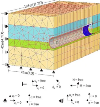
The package Plaxis 3D Tunnel is used to simulate the TBM tunneling process. Half of the domain is modeled. The outer boundaries are placed far from the tunnel to eliminate their effects on the modeling results. The numerical model has a 45 m (5D) width, a 42 m (4.7 D) height, and a 105 m (11.7 D) length (Fig. 4). A hardeningsoil material is applied for the geomechanical soil behavior. The soil layers are modeled as the hardening soil material. This model simulates the behavior of both soft soils, and stiff soils. When exposed to primary deviatoric loading, the soil shows a decreasing stiffness and simultaneously the irreversible plastic strains develop. In the special case, the observed relation between the axial strain and the deviatoric stress can be approximated by a hyperbola [45]. The structural properties are simulated as linear elastic material. The shield is modeled using the solid elements with Flexural stiffness (EI) of 8.38e4 kNm2/m, the bulk weight of 38.15 kN/m/m, and normal
stiffness (EA) of 8.2e6kN/m. The excavation round length is 1.5 m, which is equal to the tunnel segment width. The segments are simulated with Young’s modulus of 30GPa, the density of 24 kN/m3, and Poison’s ratio
of 0.2.
Fig. 4. The FEM model and the boundary conditions.
5.
Estimation of Geotechnical parameters
5.1. General
This paper discusses different approaches of estimating the settlement trough width such as empirical methods, field settlement data, and numerical solution. One of the main challenges for numerical
modeling is the accuracy of the soil parameters. For this purpose, firstly, Taguchi’s DOE was used for proper estimation of the geotechnical parameters (including E1, E2, E3, c1, c2, c3, φ1, φ2, and φ3) associated with
the soil three layers. The optimized geotechnical parameters were then used to perform a 3D numerical study for estimation of the STW parameter.
5.2. Taguchi’s Design of experiment (Taguchi’s DOE)
Taguchi’s approach is a statistical method proposed by Genichi Taguchi for assessing the influence of different parameters on the variance of the performance properties [36]. In this paper, Taguchi’s DOE was used to optimize the geotechnical parameters with a minimum number of experiments.
General steps in Taguchi’s DOE method for such geotechnical subjects are as follows:
1. determination of the Test Index (TI): the deviation of the numerical results from the filed settlement data (Settlement points C1, C2, C2L, C2R
and C3 in Table 1);
2. selection of design factors: (E1, E2, E3, c1, c2, c3, φ1, φ2, and φ3);
3. designation of the parameter levels: I, II and III (table 2); 4. running the experiments based on the orthogonal array (OA): aMINITAB program was used to compose the OA table (Table 3);
5. the numerical simulation of the experiments (models) by 3D FEM; and
6. optimization of the geotechnical parameters and selecting their best combination.
The Test Index (TI) should be calculated based on the input parameters. In this study, TI is defined as the deviation of the filed settlement data (C1, C2, C2L, C2R, C3) to the numerical results. In this
case, TI is defined as:
TI = E(p) = √1
n∑ (
uim(p)−ui
ui )
2 n
i=1 (Eq. 1)
where ui and uim(P), i = 1,2,...,n are the measured and corresponding
calculated numerical results, respectively, and n is the number of measurement points. The design factors and their levels are summarized in Table 2. The geotechnical parameters were obtained from the soil mechanic tests.
Table 2. Design factors with their values at three levels Design factors
Factor
levels E1 E2 E3 c1 c2 c3 φ1 φ2 φ3
° ° ° (kPa) (kPa) (kPa) (MPa) (MPa) (MPa) 24 28 32 24 30 14 20 30 60 I 28 30 34 28 32 16 30 40 70 II 32 32 36 32 34 18 40 50 80 III
AL27 orthogonal array was adapted for the experiments. The
lower-the-better analysis was used as the main objective of this research to reduce the deviation of the modeling results from the field measurement data. Taguchi’s L27 orthogonal design is shown in Table 3.
A total of 27 numerical models were created according to 27 Taguchi’s experiments using the geotechnical parameter combinations. For example, in experiment No.12 there are E1 = 70, E2 = 50, E3 = 30, c1 =
14, c2 = 34, c3 = 32, φ1 = 34, φ2 = 28, and φ3 = 24. After running the models,
the settlement results of numerical analysis corresponding to field settlement pins (C1, C2, C2L, C2R, C3) were calculated. Then, TI was
calculated for all experiments according to the error function Eq. 1, (the last row in table 2).
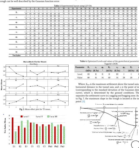
The main effect plot for test indexes average for each design factors is illustrated in Fig. 5. If we set the minimum value to the TI average, the optimal value for each design factor is obtained. For example, the c1
parameter is optimum in II level, and φ2 in I level. To find the optimal
level of the geotechnical parameters, the TI mean of geotechnical parameters for three levels, I, II and III are illustrated in Fig. 6. According to Fig. 5 and Fig. 6, the least TI mean for E1 occurs in level III, for E2 in
level II, and for E3 in level I. Similarly, the smallest TI mean for
was identified, which was selected as an optimal level for each geotechnical parameters. Thus, the optimal combination of the geotechnical parameters can be suggested as follows: E1=80, E2=40,
E3=20, c1=16, c2=34, c3=32, φ1=34, φ2=28, and φ3=32. The optimal
geotechnical parameters are presented in Table 4.
6.
Settlement Trough Width (STW) parameter
6.1.Empirical methods
The proposed empirical methods to predict the surface settlement is based on Peck’s studies (1969). According to Peck, transverse settlement trough can be well described by the Gaussian function error:
(Eq. 2)
𝑆𝑚𝑎𝑥=
𝑉𝐿
𝑖𝑥.√2𝜋 (Eq. 3)
Where Smax is the maximum settlement above the tunnel axis; x is the
horizontal distance to the tunnel axis; and ix is the point of inflection
(corresponding to the standard deviation of the Gaussian distribution curve), which is determined by the ground conditions. This point separates the settlement curve in a sagging and hogging zone. According to Fig. 7, the maximum slope in the trough is located at the inflection point [2].
Table 3. Experimental layout using L27 OA.
Experiments 1 2 3 4 5 6 7 8 9 10 11 12 13 14 15 16 17 18 19 20 21 22 23 24 25 26 27
E1 I I I I I I I I I II II II II II II II II II III III III III III III III III III
60 60 60 60 60 60 60 60 60 70 70 70 70 70 70 70 70 70 80 80 80 80 80 80 80 80 80
c1 I I I II II II III III III I I I II II II III III III I I I II II II III III III
14 14 14 16 16 16 18 18 18 14 14 14 16 16 16 18 18 18 14 14 14 16 16 16 18 18 18
φ1 32 32 32 34 34 34 36 36 36 I I I II II II III III III 34 II 34 34 36 36 36 32 32 32 36 36 36 32 II II III III III I I I III III III I 32 I 32 34 34 34 I II II II
E2 I I I II II II III III III III III III I I I II II II II II II III III III I I I
30 30 30 40 40 40 50 50 50 50 50 50 30 30 30 40 40 40 40 40 40 50 50 50 30 30 30
c2 I II III I II III I II III I II III I II III I II III I II III I II III I II III
30 32 34 30 32 34 30 32 34 30 32 34 30 32 34 30 32 34 30 32 34 30 32 34 30 32 34
φ2 I II III I II III I II III II III I II III I II III I III I II III I II III I II
28 30 32 28 30 32 28 30 32 30 32 28 30 32 28 30 32 28 32 28 30 32 28 30 32 28 30
E3 20 30 40 20 30 40 20 30 40 I II III I II III I II III III 40 20 30 40 20 30 40 20 30 30 40 20 30 I II III I II III I II II III I II III 40 20 30 40 20 I II III I
c3 24 28 32 28 32 24 32 24 28 I II III II III I III I II 24 I 28 32 28 32 24 32 24 28 24 28 32 28 II III II III I III I II I II III II III 32 24 32 24 28 I III I II
φ3 24 28 32 28 32 24 32 24 28 I II III II III I III I II 28 II III 32 24 32 24 28 24 28 32 32 24 28 24 I III I II I II III III I II I 28 II III 32 28 32 24 II III I
Test Index 5.3 9.7 7.1 5.9 5.3 5.7 7 9.9 11.2 9.5 4.8 4.2 5.1 3.8 3.1 6.5 4.7 4 4.2 6.8 3.2 3.2 4.97 3.6 3.7 3.4 4
Fig. 5. Mean effect plot for TI mean.
Fig. 6. The TI Mean for geotechnical parameters.
Table 4. Optimized Levels and values of the geotechnical parameters by Taguchi’s DOE.
3 φ 3 c 3 E 2 φ 2 c 2 E 1 φ 1 c 1 E Parameter
° (K Pa) (M Pa) °
(K Pa) (M Pa) ° (K Pa) (MPa)
III III I I III II II II III Level
32 32 20 28 34 40 34 16 80 Value
Where Smax is the maximum settlement above the tunnel axis; x is the
horizontal distance to the tunnel axis; and ix is the point of inflection
(corresponding to the standard deviation of the Gaussian distribution curve), which is determined by the ground conditions. This point separates the settlement curve in a sagging and hogging zone. According to Fig. 7, the maximum slope in the trough is located at the inflection point [2].
The inflection point (i) determines the width of the settlement trough. Peck (1969) proposed Eq. 4 to estimate the inflection point based on the tunnel depth z0 and tunnel diameter D, depending on ground
conditions:
n= 0.8-1.0 (Eq. 4) Peck (1969) established a non-dimension relation between the depth to tunnel diameter ratio (z0/D) and inflection point to tunnel diameter
ratio (2i/D) based on the field measurement in tunneling projects for different soils (Fig. 8) [2].
After the suggestion by Peck (1969), Farmer & Attewell (1974) suggested Eq. 5 for the UK tunnels based on field observations [4].
(Eq. 5) i / R = (Z0 / 2R)
Cording and Hansmire (1975) suggested a normalized relation of i-parameter, 2i/D, versus the tunnel depth, Z0/D for tunnels driven
through different geological conditions (Eq. 6).
(Eq. 6) 2i / D = (Z0 / D)0.8
Fig. 8. The relation between the settlement trough width and the tunnel’s depth for different soils [2].
Atkinson and potts (1977) presented Eq. 7 and Eq. 8 for i-parameter by examination of the field observations data and laboratory physical model tests [5].
Eq. 7 loose sand
i = 0.25 (1.5 Z0 + 0.5 R)
Eq. 8 dense sand and OC clay
i = 0.25(Z0 + 0.5 R)
Also, Glossop (1978) [6] and Mair et al. (1981) [7] are proposed Eq. 9 to estimate the i-parameter.
i = 0.5 Z0 Eq. 9
Schmidt and Clough (1981) proposed Eq. 10 for determining the inflection point to tunnel excavation by shielded machines in clays [47].
i/R =(Z0 /2R) 0.8 Eq. 10
O'Reilly and New (1982) presented 19 case studies of tunneling projects in clay and plotted i-parameter versus the corresponding tunnel depth z0. From the linear regression, they obtained the Eq. 11 for the
cohesive soil and Eq. 12 for the granular soil [8].
Eq. 11 3 ≤ Z0 ≤ 34
i = 0.43 z0 + 1.1
Eq. 12 6 ≤ Z0 ≤ 10
i = 0.28 z0 - 0.1
Herzog in 1985 suggested that the inflection point of the settlement trough can be obtained as Eq. 13 for excavation of all types of soils [9].
Eq. 13 i = 0.4 z0 + 1.92
Leach (1985) analyzed data from 23 tunnels constructed by different methods (no-shield, shield, and shield in free air, mini-tunnel, and shield in compressed air) in sites where consolidation effects are insignificant
consolidation effects are significant [48].
Eq. 14 i = 0.57 + 0.45 (z0 – z) ± 1.01
Eq. 15 i = 0.64 + 0.48 (z0 – z) ± 1.01
Kimura and Mair (1981) [49] and Fujita et al. (1982) [50] presented results from laboratory centrifuge tests. They indicated that a value of i = 0.5 z0 is obtained independently from the degree of support within the
tunnel.
Rankin (1988) reported his results from field observations of the tunnel construction but with an enlarged database and confirmed the i-value to be equal to 0.5 z0[10].
Based on the field measurement data, Arioglu (1992) found the relations for the point of inflection. He suggested Eq. 16 for excavation of clays by shield machines, Eq. 17 for excavation of all types of soils, and for excavation of all types of soils by shield machines (Eq. 18) [11].
Eq. 16 Eq. 17
Eq. 18
Mair et al. (1993) analyzed the ground deformations from tunnels in clays as well as the centrifuge tests in clay. They indicated that the subsurface settlement can also be reasonably approximated by a Gaussian error function and the i-parameter is equal to [51]:
Eq. 19 i = K (z – z0)
They observed that the i-value for subsurface settlement is significantly larger than it would be predicted with a constant K. Therefore, they suggested Eq. 20 for K [51]:
Eq. 20
Mair and Taylor (1997) reported many field data of tunneling projects with different linear regressions for tunnels in clays, sands, and gravels. As shown in Fig. 9, the i-value is varying between 0.4 and 0.6, with a mean value of K = 0.5. However, they calculated that the K ranges between 0.25 and 0.45, with a mean value of 0.35 for sandy soils [12].
(a)
Fig. 9. The inflection point (i-value) a) in clays, b) in sands and gravels [12].
Moh et al. (1996) [52] analyzed tunnels in loose sands and Dyer et al. (1996) [53] in silty sands. They obtained similar relation to Mair et al. (1993). Lee et al. (1999) reported results of 12 centrifuge tests and presented the Eq. 21 for i-parameter [13]:
Eq. 21
Hamza et al. (1999) proposed Eq. 22 for calculation of the i-value above tunnels in cohesive soil by shielded mechanics [14].
Eq. 22 i = 0.43 Z0 + 1.1
In all empirical methods, z0: tunnel depth, R: tunnel radius, z: depth
of the settlement curve and D: tunnel diameter.
Based on the literature, different authors presented various empirical equations to estimate the settlement inflection point (i-parameter). These relations are based on field measurement data, and centrifuge and physical tests in various geology conditions.
First, considering the geology conditions in understudy site, the point of inflection in the settlement trough is calculated based on the empirical approaches.
In this section, the tunnel’s diameter is 9.14 m; the tunnel’s radius is 4.55 m, and the depth of tunnel is 15.5 m.
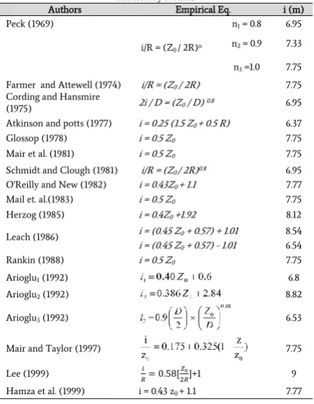
The calculated i-value based on the empirical formulas presented in Table 5 (right column). The maximum i-value is 9 m, which is obtained by Lee’s formula (1999). The minimum i-value is 6.37 m that is calculated by Atkinson and Potts’ formula (1977).
Table 5. The settlement point inflection based on the empirical formula in understudy section.
i (m) Empirical Eq.
Authors
6.95 n1 = 0.8
i/R = (Z0 / 2R)n Peck (1969)
7.33 n2 = 0.9
7.75 n3 =1.0
7.75 i/R = (Z0 / 2R)
Farmer and Attewell (1974)
6.95 2i / D = (Z0 / D) 0.8
Cording and Hansmire (1975)
6.37 i = 0.25 (1.5 Z0 + 0.5 R)
Atkinson and potts (1977)
7.75 i = 0.5 Z0
Glossop (1978)
7.75 i = 0.5 Z0
Mair et al. (1981)
6.95 i/R = (Z0 / 2R)0.8
Schmidt and Clough (1981)
7.77 i = 0.43Z0 + 1.1
O'Reilly and New (1982)
7.75 i = 0.5 Z0
Mail et. al.(1983)
8.12 i = 0.4Z0 +1.92
Herzog (1985)
8.54 i = (0.45 Z0 + 0.57) + 1.01
Leach (1986)
6.54 i = (0.45 Z0 + 0.57) - 1.01
7.75 i = 0.5 Z0
Rankin (1988)
6.8 Arioglu1 (1992)
8.82 Arioglu2 (1992)
6.53 Arioglu3 (1992)
7.75 Mair and Taylor (1997)
9
𝑖
𝑅= 0.58[
𝑍0
2𝑅]+1
Lee (1999)
7.77 i = 0.43 z0 + 1.1
Hamza et al. (1999)
The settlement trough form is given by Peck’s equation (Eq. 1). Two parameters are determining the shape and magnitude of the trough: the point of inflection (i-parameter) and the volume loss VL (see Fig. 10).
Volume loss (VL) is the ratio of the difference between the excavated
volume of soil and the tunnel’s volume (defined by the tunnel's outer
diameter) over the tunnel’s volume.
Fig. 10. The point of inflection and the volume loss in the settlement curve. The VL value was determined based on the excavation method,
technical details of the drilling machine, and the tunneling experiments in similar geotechnical conditions. This parameter was between 1% and 2% according to Mair (1999) for tunneling in clay soils using the closed shields. VL considered a 1% for tunneling with EPB TBM [12].
For plotting the settlement curve based on the empirical i-value, the known values (i and VL) were assigned to the Eq. 1 (the VL = 1% and i =
calculated i-value for each author based in Table 5). Therefore, the settlement formula was obtained, and the settlement curve could be plotted. For example, in Glossop’s relation (1978) (the VL = 1% and i =
7.5m), the settlement formula is calculated as follows:
Thus, the settlement curve can be plotted based on assigning the value to x. The plotted settlement trough based on the empirical i-values is illustrated in Fig. 11.
Fig. 11. The settlement trough based on the empirical i-values.
We consider the mean of empirical methods for estimation of standard deviation, i-value:
𝑖 =𝑖1+ 𝑖2+ ⋯ + 𝑖𝑛
𝑛 = 7.58
center. The matching of the center of the inflection zone with the mean of the empirical i-values indicates that the averaging of all the empirical i-values is relatively correct assumption to estimate the inflection point width.
6.2. Field instrument data
After calculation of the inflection point (i-value), according to the empirical formulas, we investigated the i-value estimation based on the field instrument data. There are two approaches to evaluate the point of inflection:
1. Using a linear regression to calculate the gradient of the plot of ln S/Smax versus x2 for each settlement profile, and the value of the gradient
is equal to (-1/ (2i2)).
2. Establishing the change in the slope of the computed settlement profile.
Based on the first approach, the settlement profile is predicted as the error function curve (Eq.2); taking a natural log from the above Eq.2 gives Eq. 23:
ln 𝑆 = ln 𝑆𝑚𝑎𝑥(−
𝑥2
2𝑖2) ⇒ 𝑖 = √
𝑥2
2 ln ( 𝑆
𝑆𝑚𝑎𝑥)
Eq. 23
By plotting ln(S/Smax) versus 𝑥2, the gradient obtained would be equal
to − 1
2𝑖2, and i-value can be evaluated. The field settlement data onto
understudy zone are summarized in table 1. For calculation of i-value based on the field measurement data onto C2 section: Smax = SC2 = 46.7
mm; S = SC2L = 29 mm; x = 7.5 m:
𝑖 = √2 ln (𝑥2𝑆
𝑆𝑚𝑎𝑥)
= √2 ln (7.50.0292
0.046)
= 7.68 𝑚
The settlement trough width curve of the field measurement data is illustrated in Fig. 12. In this paper, the distance between the tunnel’s centerline and the point of the settlement is less than 0.5 mm considered as the STW parameter. As shown in Fig. 15, the STW parameter is 23 m (equal to 3i). The calculated i-value using the field measurement data is closer to the obtained i-value from empirical approaches. This shows the good agreement between the field measurement data and the empirical methods.
6.3. Numerical solution
The optimized geotechnical parameters are applied for tunneling simulation by the FEM analysis for estimation of the STW parameter. We applied the real conditions of the tunneling project in the numerical modeling simulation. The results of the numerical modeling are illustrated in Fig. 13. The STW parameter is 27 m. Considering that the STW parameter is equal to 3i, the i-value is equal to 9 m. The Fig. 16 indicated that the numerical modeling leads to a wider STW parameter than those of the field settlement data and empirical methods.
Fig. 12. The settlement trough curve based on the field measurement data.
Fig. 13. The settlement trough curve based on the numerical modelling.
The results of the numerical modeling, field measurement data, and empirical approaches is illustrated in Fig. 14. The STW parameter is equal to 7.58 m, 7.68 m, and 9 m for empirical methods average, field settlement data and numerical analysis, respectively.
Fig. 14 indicates that the calculated i-value from empirical methods average has a good agreement with the calculated i-value from field measurement data, despite the considerable difference in the maximum settlement. The FEM numerical analysis overestimated the STW parameter compared to the results of field instrument data and empirical methods.
Fig. 14. The settlement trough based on the numerical modeling, field measurement data, and empirical approaches.
Conclusion
equal 7.58 m and the STW parameter is 22.8 m. The i-value was calculated to be 23 m using the field settlement date. The numerical results lead to extent the settlement trough to 27 m. The results indicate that Taguchi’s (DOE) method is an effective approach to estimate the geotechnical parameters. The numerical modeling gives a wider settlement trough than those of the empirical methods and instrument data. However, the numerical modeling has a minimal error in the field measurement data. There is a good agreement between the calculated STW parameter by empirical formula and field settlement data. The numerical simulation overestimated the STW parameter. It causes more buildings to be included in the tunnel impact zone. It demands more extensive study to assess the tunneling-induced building damage, which is more conservative.
REFRENCES
[1] Nations, U., World Urbanization Prospects: The 2014 Revision, Highlights. Department of Economic and Social Affairs. Population Division, United Nations, 2014.
[2] Peck, R.B., Deep excavations and tunneling in soft ground. Proc. 7th Int. Con. SMFE, State of the Art, 1969: p. 225-290.
[3] Schmidt, B., A method of estimating surface settlement above tunnels constructed in soft ground. Can Geotech J, 1969. 20: p. 11-22.
[4] Attewell, P. and I. Farmer, Ground deformations resulting from shield tunnelling in London Clay. Canadian Geotechnical Journal, 1974. 11(3): p. 380-395.
[5] Atkinson, J.H. and D.M. Potts, Subsidence above shallow tunnels in soft ground. Journal of Geotechnical and Geoenvironmental Engineering, 1977. 103(Proc. Paper 11318 Proceeding).
[6] Glossop, N.H., Soil deformations caused by soft-ground tunnelling. 1978, Durham University.
[7] Mair, R., M. Gunn, and M. O'REILLY, Ground movement around shallow tunnels in soft clay. Tunnels & Tunnelling International, 1982. 14(5).
[8] O'reilly, M. and B. New, Settlements above tunnels in the United Kingdom-their magnitude and prediction. 1982.
[9] Herzog, M., Surface subsidence above shallow tunnels. Bautechnik, 1985. 62(11): p. 375-377.
[10] Rankin, W., Ground movements resulting from urban tunnelling: predictions and effects. Geological Society, London, Engineering Geology Special Publications, 1988. 5(1): p. 79-92.
[11] Arioglu, E., Surface movements due to tunnelling activities in urban areas and minimization of building damages. Short Course, Istanbul Technical University. Mining Engineering Department (in Turkish), 1992.
[12] Mair, R. and R. Taylor. Theme lecture: Bored tunneling in the urban environment. in Proceedings of the fourteenth international conference on soil mechanics and foundation engineering (Hamburg, 1997), Balkema. 1999.
[13] Lee, K., et al., Ground response to the construction of Shanghai metro tunnel-line 2. Soils and Foundations, 1999. 39(3): p. 113-134. [14] Hamza, M., A. Ata, and A. Roussin, Ground movements due to the construction of cut-and-cover structures and slurry shield tunnel of the Cairo Metro. Tunnelling and Underground Space Technology, 1999. 14(3): p. 281-289.
[15] Taguchi, G. and G. Taguchi, System of experimental design; engineering methods to optimize quality and minimize costs. 1987.
[16] Daneshvar, N., et al., Biodegradation of dye solution containing Malachite Green: Optimization of effective parameters using Taguchi method. Journal of Hazardous Materials, 2007. 143(1): p. 214-219.
[17] Delgado-Moreno, L., A. Pena, and M. Mingorance, Design of experiments in environmental chemistry studies: Example of the extraction of triazines from soil after olive cake amendment. Journal of hazardous materials, 2009. 162(2): p. 1121-1128. [18] Sutcu, M., et al., Effect of olive mill waste addition on the
properties of porous fired clay bricks using Taguchi method. Journal of environmental management, 2016. 181: p. 185-192. [19] Rasoulifard, M.H., M. Akrami, and M.R. Eskandarian, Degradation
of organophosphorus pesticide diazinon using activated persulfate: Optimization of operational parameters and comparative study by Taguchi's method. Journal of the Taiwan Institute of Chemical Engineers, 2015. 57: p. 77-90.
[20] Ng, E.Y. and W.K. Ng, Parametric study of the biopotential equation for breast tumour identification using ANOVA and Taguchi method. Medical and Biological Engineering and Computing, 2006. 44(1-2): p. 131-139.
[21] Taguchi, K., et al., Effect of albumin on transthyretin and amyloidogenic transthyretin Val30Met disposition and tissue deposition in familial amyloidotic polyneuropathy. Life sciences, 2013. 93(25): p. 1017-1022.
[22] Kurmi, M., et al., Implementation of design of experiments for optimization of forced degradation conditions and development of a stability-indicating method for furosemide. Journal of pharmaceutical and biomedical analysis, 2014. 96: p. 135-143. [23] Sánchez-López, E., et al., PEGylated PLGA nanospheres
optimized by design of experiments for ocular administration of dexibuprofen—in vitro, ex vivo and in vivo characterization. Colloids and Surfaces B: Biointerfaces, 2016. 145: p. 241-250. [24] Dawud, E.R. and A.K. Shakya, HPLC-PDA analysis of
ACE-inhibitors, hydrochlorothiazide and indapamide utilizing design of experiments. Arabian Journal of Chemistry, 2014.
[25] Siyal, A.A., et al., Effects of Parameters on the Setting Time of Fly Ash Based Geopolymers Using Taguchi Method. Procedia Engineering, 2016. 148: p. 302-307.
[26] Tchognia, J.H.N., et al., Application of Taguchi approach to optimize the sol–gel process of the quaternary Cu 2 ZnSnS 4 with good optical properties. Optical Materials, 2016. 57: p. 85-92. [27] Tučková, M., et al., Design of experiment for hysteresis loops
measurement. Journal of Magnetism and Magnetic Materials, 2014. 368: p. 64-69.
[28] Wu, C.-H. and W.-S. Chen, Injection molding and injection compression molding of three-beam grating of DVD pickup lens. Sensors and Actuators A: Physical, 2006. 125(2): p. 367-375. [29] Kitchen, R.R., M. Kubista, and A. Tichopad, Statistical aspects of
quantitative real-time PCR experiment design. Methods, 2010. 50(4): p. 231-236.
[30] Li, M., et al., Simulation-based experimental design and statistical modeling for lead time quotation. Journal of Manufacturing Systems, 2015. 37: p. 362-374.
[31] Mamourian, M., et al., Optimization of mixed convection heat transfer with entropy generation in a wavy surface square lid-driven cavity by means of Taguchi approach. International Journal of Heat and Mass Transfer, 2016. 102: p. 544-554. [32] Romero-Villafranca, R., L. Zúnica, and R. Romero-Zúnica,
[33] Azadeh, A., et al., A hybrid fuzzy mathematical programming-design of experiment framework for improvement of energy consumption estimation with small data sets and uncertainty: The cases of USA, Canada, Singapore, Pakistan and Iran. Energy, 2011. 36(12): p. 6981-6992.
[34] Chompu-inwai, R., B. Jaimjit, and P. Premsuriyanunt, A combination of Material Flow Cost Accounting and design of experiments techniques in an SME: the case of a wood products manufacturing company in northern Thailand. Journal of Cleaner Production, 2015. 108: p. 1352-1364.
[35] Elshennawy, A.K., Quality in the new age and the body of knowledge for quality engineers. Total Quality Management & Business Excellence, 2004. 15(5-6): p. 603-614.
[36] Balki, M.K., C. Sayin, and M. Sarıkaya, Optimization of the operating parameters based on Taguchi method in an SI engine used pure gasoline, ethanol and methanol. Fuel, 2016. 180: p. 630-637.
[37] Lai, F.-M. and C.-W. Tu, Optimizing the manufacturing parameters of carbon nanotubes stiffened speaker diaphragm using Taguchi method. Applied Acoustics, 2016. 113: p. 81-88. [38] Rao, R.S., et al., The Taguchi methodology as a statistical tool for
biotechnological applications: a critical appraisal. Biotechnology journal, 2008. 3(4): p. 510-523.
[39] Roy, R.K., Design of experiments using the Taguchi approach: 16 steps to product and process improvement. 2001: John Wiley & Sons.
[40] Ozcelik, B. and T. Erzurumlu, Comparison of the warpage optimization in the plastic injection molding using ANOVA, neural network model and genetic algorithm. Journal of materials processing technology, 2006. 171(3): p. 437-445.
[41] Rieben, E.H., Geological observations on alluvial deposits in northern Iran. 1966: Geological Survey of Iran.
[42] Pedrami, M., Pasadenian orogeny and geology of last 700,000 years of Iran. Geological Survey of Iranin, 1981.
[43] Fakher, A., A. Cheshomi, and M. Khamechiyan, The addition of geotechnical properties to a geological classification of coarse-grained alluvium in apediment zone. Quarterly journal of engineering geology and hydrogeology, 2007. 40(2): p. 163-174. [44] Corporation, S.C.E., [5] Geotechnical and geology
engineering investigation of Metro Line 7, East- West route. 2009. [45] Duncan, J.M. and C.-Y. Chang, Nonlinear analysis of stress and strain in soils. Journal of Soil Mechanics & Foundations Div, 1970. [46] Leca, E. and B. New, Settlements induced by tunneling in soft ground. Tunnelling and Underground Space Technology, 2007. 22(2): p. 119-149.
[47] Clough, G.W., Design and performance of excavations and tunnels in soft clay. In Soft Clay Engineering, 1981: p. 569-634. [48] Leach, G., Pipeline response to tunneling. Unpublished paper,
1985.
[49] Kimura, T. and R. Mair. Centrifugal testing of model tunnels in soft clay. in Proceedings of the 10th international conference on soil mechanics and foundation engineering. 1981. ISSMFE: International Society for Soil Mechanics and Foundation Engineering.
[50] Fujita, K. Prediction of surface settlements caused by shield tunnelling. in Proceedings of the international conference on soil mechanics. 1982.
[51] Mair, R., R. Taylor, and A. Bracegirdle, Subsurface settlement profiles above tunnels in clays. Geotechnique, 1993. 43(2). [52] Moh, Z., D.H. Ju, and R. Hwang. Ground movements around
tunnels in soft ground. in Proceedings International Symposium on Geotechnical Aspects of Underground Construction in Soft Ground. 1996. London: Balkema AA.