Glacier Biogeochemistry

(1)

Volume 6, number 2 | October 2017

MAR

TIN

S

HAR

P

MAR

T

YN

TR

AN

TE

R

_Glacier

(2)

L

iane

G. B

enninG

GFZ Potsdam, Germany University of Leeds, UK

S

teven

a. B

anwart

University of Leeds, UK

Editorial Board

t

im

e

LLiott

University of Bristol, UK

D

on

C

anfieLD

University of Southern Denmark, Denmark

S

uSan

L.S. S

tipp

University of Copenhagen, Denmark

Editorial Manager

m

arie

-a

uDe

H

uLSHoff

Graphical Advisor

J

uan

D

ieGo

r

oDriGuez

B

LanCo

Trinity College Dublin, Ireland Each issue of Geochemical Perspectives

pre-sents a single article with an in-depth view on the past, present and future of a field of geochemistry, seen through the eyes of highly respected members of our community. The articles combine research and history of the field’s development and the scientist’s opinions about future directions. We welcome personal glimpses into the author’s scientific life, how ideas were generated and pitfalls along the way.

Perspectives articles are intended to appeal to the entire geochemical community, not only to experts. They are not reviews or monographs; they go beyond the current state of the art, providing opinions about future directions and impact in the field.

Copyright 2017 European Association of Geochemistry, EAG. All rights reserved. This journal and the individual contributions contained in it are protected under copy-right by the EAG. The following terms and conditions apply to their use: no part of this publication may be reproduced, translated to another language, stored in a retrieval system or transmitted in any form or by any means, electronic, graphic, mechanical, photo-copying, recording or otherwise, without prior written permission of the publisher. For information on how to seek permission for reproduction, visit:

www.geochemicalperspectives.org

or contact [email protected]. The publisher assumes no responsibility for any statement of fact or opinion expressed in the published material.

ISSN 2223-7755 (print) ISSN 2224-2759 (online) DOI 10.7185/geochempersp.6.2

Principal Editor for this issue Liane G. Benning Reviewers

Marek Stibal, Charles University, Czech Republic Rob Raiswell, University of Leeds, UK Cover LayoutPouliot Guay Graphistes

TypesetterInfo 1000 Mots

PrinterDeschamps impression About the cover_{A frozen cryolake on the surface of Canada} Glacier, which is located in Taylor Valley, Antarctica.

Photo credit: Martyn Tranter

J

anne

B

LiCHert

-t

oft

(3)

PREFACE

Martin (MS) and I (MT) have been encouraged to write this volume of Geochem-ical Perspectives in a travelogue style, sketching out the research terrain we entered and encountered as post-graduates, and then relating why we tackled particular problems in the order we did. We have been encouraged to acknowledge the wisdom of our mentors, peers, post-docs and post-graduates along the journey, which has been a great pleasure. We feel we are nowhere near our final desti-nation as yet – there are paradigm shifts occurring in the field of glacier biogeo-chemistry even as we write – and we hope that this is a stimulus for early career researchers who may read this manuscript. We further hope that the story of the origins of the study of glacier biogeochemistry that we narrate will capture your imagination, as it did ours, and that we can convince you that glaciers and ice sheets are important and dynamic components of the Earth system.

(8)

Martin Sharp (MS) Earth and Atmospheric Sciences University of Alberta Edmonton, Alberta T6G 2E3, Canada

(9)

GLACIER

BIOGEOCHEMISTRY

_ABSTRACT

(10)

(11)

1. INTRODUCTION – HOW WE GOT INTO GLACIER

_{HYDROLOGY AND HYDROCHEMISTRY IN THE 1970’S}

1.1 First Steps (MS)

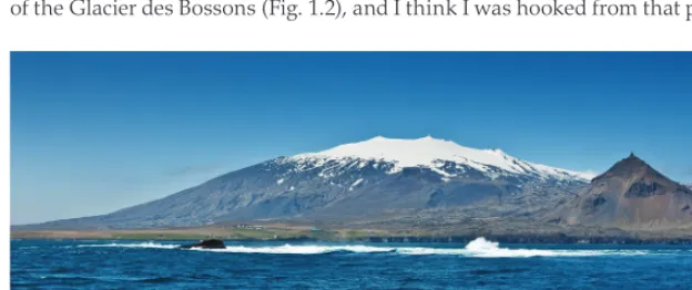
I saw my first glacier in Iceland in 1973 on a school field trip. It was the ice cap on top of Snaefell in Iceland – in literature, it is the start of the Jules Verne’s Journey to the Centre of the Earth, which, with the benefit of hindsight, seems more prophetic than I imagined at the time (Fig. 1.1). The next year, I had the chance to visit Chamonix, a place that plays an important role in the early annals of glaci-ology and is site of some of the earliest in situ subglacial science – in the tunnel beneath the Glacier d’Argentière. On that visit, I got to explore along the margins of the Glacier des Bossons (Fig. 1.2), and I think I was hooked from that point on.

Figure 1.1 Snaefellsjokull, Iceland – Martin’s first glacier, and the starting point for the Journey to the Centre of the Earth.

In 1976, I went to Cambridge University to study Geography, and in 1978 I had to produce a thesis for my degree program. This seemed like a good chance to go back to Iceland and spend more time around glaciers. With encouragement from Helgi Björnsson, one of the pioneers of modern glacier hydrology, I surveyed a long profile up the centre of the surge-type glacier, Sylgjujökull, on the west side of the ice cap Vatnajökull, and made a study of the shorelines developed around a former surge-dammed lake.

(12)

Figure 1.2 Glacier des Bossons, Chamonix, France, where Martin got hooked on glaciers.

(13)

theme in this narrative) on a series of exposures that seemed to show that, during a previous surge, the glacier had moved over extremely wet sediments that had been liquefied by the loading pressure of the advancing glacier. Deformation of those sediments played an important role in landform building and probably also contributed to the motion of the overlying ice (an idea that was just starting to emerge in the literature through the work of Geoffrey Boulton). This kick-started my fascination with the interactions between glaciers and the water that was trying to drain over, through and beneath them.

1.2 Next Steps – the New World (MS)

After leaving Aberdeen, I was fortunate to win a Junior Research Fellowship at Merton College, Oxford, to study the dynamics of surge-type glaciers. I was even more fortunate that the then Warden, Rex Richards, was willing to give me the freedom to spend significant parts of my Fellowship working elsewhere to develop my knowledge, skills, and experience. This allowed me to spend 6 months at the University of Washington (UW) in Seattle, under the tutelage of Bernard Hallet and Charlie Raymond, who were both great mentors. At the time, UW was an incredibly dynamic environment for anyone interested in glaciers, and many of those I mixed with have gone on to become leaders in their fields – in particular, Bob Anderson, Andrew Fountain, Tad Pfeffer, Joe Walder, Tómas Johannesson and Magnus Magnusson. It has been my pleasure to continue rela-tionships with many of them ever since. The highlight of this first visit to North America was spending the summer of 1983 on Variegated Glacier, near Yakutat in southern Alaska (Fig. 1.4). It was being monitored in the build-up to a surge that was expected to occur sometime in the mid-1980’s – but it conveniently started to surge in the winter of 1982-1983.

(14)

had accomplished a lot of erosion of the glacier’s bed. By this time, there was no way I was going to work on anything other than the interactions between glacier flow, glacier hydrology, and subglacial geomorphological processes. Meltwater chemistry, however, had yet to trouble my consciousness.

Figure 1.4 Alaska’s Variegated Glacier during its 1983 surge.

1.3 Back to Cambridge (MS)

While on the glacier, I received a message from Bernard Hallet that there was a faculty position in Physical Geography available at Cambridge University and that I was encouraged to apply for it. Barclay agreed that if I produced a CV he would take it with him when he left the glacier and send it to Cambridge for me. It was nearing the end of the season, field books were more or less full, and personal computers had yet to be invented, so I hand wrote my CV on the inside of a breakfast cereal box. Barclay didn’t bat an eyelid, and somehow the CV found its way to Dick Chorley in Cambridge (whether still on the cereal box or not I never found out, though Dick would probably have appreciated it all the more if it had been!). When I returned to the UK, I was called for interview and was extremely lucky to be offered the job. I returned to Cambridge in April 1984.

(15)

to retrieve a time-lapse camera and data logger that he and Joe Walder had installed in a cavity beneath the Grinnell Glacier (Fig. 1.5). For the first time, I realised that (a) it was possible to crawl long distances under some glaciers, and (b) you could do science under glaciers without the benefit of hydro-electricity tunnels or hot water drills. I also learned that there are better ways to download a data logger than spending 9 hours in the dark at 0 °C transcribing each individual data point collected in the previous 2 years into a notebook! We had planned to just pick up the logger and bring it back to Seattle for downloading – but it turned out that with this early model, disconnecting it from its power source would wipe the memory, so we did what we had to do! After escaping from Grinnell, we paid a visit to Blackfoot Glacier, where Bernard and Joe Walder had mapped, in great detail, the geomorphological evidence for patterns of subglacial water flow across the limestone bedrock now exposed in front of the glacier. This included evidence for extensive dissolution weathering of the limestone and for subglacial carbonate precipitation on the downstream side of bedrock bumps – low pressure locations when ice-covered – where water was expected to freeze, thereby concentrating the solute to the point of supersaturation and precipitation. This is where I finally got the message that there might be such a thing as glacier geochemistry and that it might, in some way, be connected to glacier hydrology.

(16)

Back in Cambridge, it was time to start a field research programme. By chance, there was another new appointment in the department – Keith Richards, not a guitarist, but a well-known fluvial geomorphologist, who was also looking for ideas for a field programme that we could use as a basis for training students (in those days Cambridge students got very little field training). We decided to pool our resources and settled on the Hardanger ice cap in southern Norway as a suitable field site – where we worked from 1985-1988. This is how I finally got into glacier hydrology. Ian Willis joined us as a Ph.D. student to work there and has now been involved in the field for nearly 30 years (as has one of the undergraduates on that first trip; Peter Nienow). Probably the most important outcome of the work in Norway was that we learned how to conduct dye tracing experiments on glaciers – our first venture into investigating how the efficiency of glacier drainage systems changes over the course of a melt season. The problem with summers in southern Norway, however, is that it rains a lot. Rain wasn’t very compatible with early 1980’s era surveying equipment or data loggers, so it was hard to generate long, unbroken series of measurements. At the end of the 1987 field season, Keith symbolically set fire to his field boots and sent them to a Viking burial in the Hardanger Fjord.

1.4 The Alps (MS)

Our thoughts turned to warmer climes and, in 1988, we decided to try to get funding for a glacier hydrological project in the Swiss Alps. We teamed up with Mike Clark and Angela Gurnell at Southampton University, who had been working in the Arolla Region and had just edited a seminal book “Glacio-fluvial Sediment Transfer: an Alpine Perspective”. It presented what was then the state of the art in the science of glacier hydrology and fluvio-glacial sediment transport, but didn’t say too much about glacier hydrochemistry – which was a fair reflec-tion of the state-of-the-science at the time – although it did contain a chapter on current thinking by Roland Souchez and Reggie Lorrain from Brussels. It was at a meeting to plan the proposal writing for this project that my life path collided with that of the more entertaining Martyn, who had recently taken up a position as a marine sedimentary geochemist in the Department of Oceanography at Southampton. I’ll let him take it from there!

1.5 First Encounters with Glacier Meltwater Geochemistry (MT)

(17)

playing cricket for Ebbw Vale. However, both Mam and Dad were keen for me to go to university, and they encouraged me to spread my wings, mix metaphors and sail to the distant flat lands of Norfolk to attend UEA.

I can’t explain why I got interested in silicate rock dissolution, particularly since silicate rocks dissolve in water very slowly, but I did. I’ve always liked puzzles and problems, and there was controversy about what stopped them dissolving more quickly. I got hung up on why one of the most common silicate minerals, feldspar, dissolves in the way it does. Feldspar surfaces initially react rapidly with water, a process known as hydrolysis, but dissolution slows down drastically thereafter. The positively charged cations in the mineral surface, such as Na+_{, K}+ _{and Ca}2+_{, are displaced by H}+_{, and leave behind a leached surface layer.} The controversy in the 1970’s was about the thickness and composition of the leached layer (or indeed whether it existed), and I was hooked on doing my own simple experiments to make a contribution to the debate.

Rob Raiswell (the co-author of the very first Geochemical Perspectives issue) taught the Year 2 Geochemistry course, was interested in this general area too, and went on to supervise my undergraduate dissertation on feldspar dissolution in distilled water in free contact with the atmosphere. Peter Brimblecombe taught me Year 3 Environmental Aquatic Chemistry. They were inspirational lecturers and great researchers. I learnt tons about CO2 and dissolved carbonate species, about pH measurement and the partial pressure of CO2 in solution, and I learnt lots about solution geochemistry. Rob was becoming interested in glacier hydro-chemistry and had a Ph.D. on offer, which included an investigation of silicate dissolution at glacier beds. There was fieldwork in the Alps. I thought that this sounded great fun, and applied for the position. I was very lucky to get the studentship, and was not a good post-graduate. I loved playing cricket and all the socialising that went with it.

Thankfully, Rob was determined to keep me on track, and largely drove me through the Ph.D., despite my kicks, screams and hedonism. He arranged my first field season in the summer of 1979 in the Swiss Alps at Gornergletscher (Fig. 1.6) with the legendary Dave Collins and his Manchester group. We sampled waters at hourly intervals during several days and nights, filtering the waters shortly after collecting them, and made pH measurements on the samples as quickly as we could. We measured cation concentrations on return to UEA by AAS (atomic absorption spectroscopy), and a big innovation was measuring the common strong acid anions, Cl-_{, NO}

(18)

Figure 1.6 Switzerland’s Gornergletscher, where Martyn got addicted to very dilute water.

We followed up with a second season at Glacier des Bossons in 1980, with my future best man, Paul Garrad, and Alun Thomas, Rob’s first Ph.D. student. They both were fantastic in the field, totally unflappable whatever the weather and despite the odd working hours we had to keep. The closest they came to revolt was when I served up a sardine curry made from leftovers one evening. We repeated our work from Gornergletscher, finding broadly similar results. Sulphate seemed to be a key ion – it was concentrated in the concentrated waters, but virtu-ally absent in the dilute waters. Writing up the work for my Ph.D. thesis revealed a few problems with using the common electrical conductivity-based mixing model that separated the runoff at the glacier terminus into two components of discharge, one that flowed rapidly from the glacier surface to the terminus and one that flowed slowly across the glacier bed. The composition of these two components could not be as constant as the literature of the time required. Rob continually nursed and kicked me through to getting my Ph.D., which was to be the last of the hand-written and hand-typed at Environmental Sciences, UEA.

(19)

quickly that you had to publish or perish. Trevor and Rob were great influences on me. They were generous with ideas, contacts and polishing my tortured writing. They instilled an attitude that collaboration and cooperative effort usually wins in the long run, a philosophy that I’ve tried to maintain ever since, despite the burns every academic feels at times. I’ve tried to be like them since with my own graduate students and post-docs, but come up very short, of course.

1.6 Southampton – Where Oceanography and Glaciology Collided

(MT)

The University sector contracted during the Thatcher cut-back years, and yet I was very fortunate to obtain a lectureship in Marine Sedimentary Geochemistry at Oceanography, Southampton, largely on the back of Rob’s international repu-tation and the hope that some of his expertise must have rubbed off on me. I fell under the mentorship of Dennis Burton, another inspirational geochemist, and was hugely influenced by my friend, Peter Statham, on the need for good meth-odology in chemical analysis. I became immersed in putting together a marine geochemistry course, establishing a marine research profile, far from my glacier and acid snow days, when, out of the blue, Angela Gurnell knocked on my door.

1.7 Our Paths Converge (MT)

(20)

2. _{GLACIER HYDROLOGY IN THE 1960’S AND 1970’S}

2.1 Early Perspectives on Glacier Hydrology and Glacier Flow (MS)

Early thinking about glacier hydrology attempted to understand the mechanisms by which glacier flow and sliding occurred. It had been long known, since the work of J.D. Forbes (Fig. 2.1) on the Mer de Glace (Chamonix) in the 1840’s, that the velocity of a glacier can vary seasonally, being higher in summer, when melt-water is abundant, and lower in winter, when meltmelt-water is either absent or much less abundant. By the 1960’s, it was also known that meltwater efflux from glacier termini varied seasonally and diurnally (in summer), more or less in parallel with variations in surface melt rates.

Early efforts at drilling and tunnelling through glaciers (e.g., Mathews, 1964) had encountered englacial water pockets, so it was clear that there had to be a meltwater drainage system within glaciers that connected the surface to the terminus. Observations in a shaft beneath Canada’s South Leduc Glacier had found variations in water pressure at the bed that were connected to the occur-rence of rainfall and melt events on the glacier surface (Mathews 1964). From the 1940’s, a number of workers made measurements of the rate of movement of glacier soles in natural cavities and tunnels, finding that there was measur-able displacement between the glacier and its bed (Carol, 1947; Haefeli, 1951; Kamb and LaChapelle, 1964). Veloc-ities measured at glacier beds were often spatially variable and always less than velocities measured nearby at the glacier surface. Surface velocities clearly varied over time and measurements of water pressure at the bed suggested that this might be connected to hydro-logically-forced fluctuations in basal friction. From these observations, it was clear that there must be at least 2 processes of glacier flow – one involving the deformation of the ice itself, and another involving displacement of the ice relative to the bed (or sliding), which might be affected by variations in the flux and pressure of subglacial water.

(21)

2.2 The Development of Theory Relating Glacier Hydrology

and Glacier Flow (MS)

The first quantitative theory of glacier sliding (Weertman, 1957) argued that sliding occurred when the ice at the bed was at the pressure melting temperature, and that it arose from the sum of two processes – regelation and enhanced viscous deformation. These are both linked to the fluctuations in ice-bed contact pressure that occur as a glacier moves past roughness elements (or bumps) on its bed.

Because the ice is at the pressure melting temperature, and the pressure is higher on the upstream side of the bump than on the downstream side, so the ice temperature on the upstream side is lower than it is on the downstream side, where pressure is lower. The resulting temperature gradient across the bump means that heat flows through the rock from the downstream side to the upstream side, causing melting on the upstream side. The water produced by this melting flows along the gradient from high to low pressure that exists across the bump. As this water is colder than the ice on the downstream side, it refreezes when it gets to the lee side of the bump. The latent heat of refreezing that is released flows back through the bump to drive melting on the upstream side. This process only works for relatively short wavelength bumps, but it creates short length-scale (from several cm to several m) meltwater drainage systems at the glacier bed, associated with topographic irregularities.

(22)

Where the bedrock is highly soluble in water (as is limestone, for instance), the meltwater in the regelation water film may dissolve the bedrock on the upstream side of a bump, transport the resulting solute around the bump to the leeside, and then precipitate it in mineral form on the leeside, where refreezing rejects solute and concentrates it to the point of supersaturation (Fig. 2.2). Since the presence of solute in the water alters the temperature at which the water will freeze, there is a feedback on both the regelation process and the flow of the glacier. Geomorphological evidence from recently deglaciated limestone surfaces supports this idea very clearly (Hallet, 1976a; Walder and Hallet, 1979; Hallet and Anderson, 1980). This is perhaps the first work to articulate clearly a coupling between subglacial hydrology, glacier flow, and subglacial geochemical processes.

2.3 Glacier Hydrochemistry in the 1970’s (MT)

The Earth Science community tended to think that much of the glacier bed was frozen to bedrock, and that the lack of water and low temperatures precluded very much chemical weathering (Gibbs and Kump, 1994). Glaciers were also thought to be biologically inert, since earth scientists and glaciologists found it very diffi-cult to believe that microbes could function in the cold and dark (Raiswell and Thomas, 1984). Glacial meltwaters that were sampled were often quite dilute (Raiswell, 1984) and, as such, they offered little of interest to geochemists at the time. However, there were a few things to interest anyone interested in dissolving sparingly soluble silicate minerals.

Glaciers are powerful agents of physical erosion, pulverising or commin-uting the bedrock they flow over, producing glacial flour. Early work on glacier meltwater geochemistry aimed to show that glacial flour produced fertile soils, because of the relative ease with which cations could be obtained by plants from the flour. Glacial meltwaters easily transport the flour and are milky as a consequence (Keller and Reesman, 1963), often containing ~1 g L-1_{of fine} suspended sediment. The grains are often mainly silt- to clay-sized (Keller and Reesman, 1963; Hallet et al., 1996), and this maximises the potential for minerals to dissolve. The meltwater chemistry of runoff from a variety of glaciers in the USA, the Alps, Norway and Antarctica could be simulated in the laboratory by grinding rocks in double distilled water. Hydrolysis, the interaction of water with the surfaces of silicate minerals such as feldspars, was thought to generate the solute (equation 2.1),

(23)

and quartz. However, carbonates yielded the most solute, because carbonate hydrolysis completely dissolves the surface of the mineral, rather than leaving behind a leached surface layer.

CaCO3 (s) + H2O (l) ↔ Ca2+ (aq) + HCO3- (aq) + OH- (aq) (2.2)

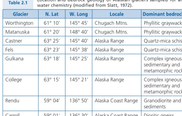
Figure 2.3 Major cation and dissolved Si concentrations in meltwaters from 9 Alaskan glaciers (modified from Slatt,1972). Figures in those days were drawn by hand, and labelling was not always as bold as brass. The Y axis is the concentration in units of ppm. The first three samples on the left come from Worthington Glacier (sampled in 1968 and 1969), the next is from Matanuska Glacier (1969), followed by three from Castner Glacier (1968 and 1969), followed by one each from Fels, Gulkana, College, Rendu, Carroll and Norris Glaciers (1969). Note that Ca2+ _{is always the dominant cation in all samples analysed (lowest white} space on column), usually folled by Mg2+_{(diagonal stripes sloping down from} the left), and that Na+ _{(vertical lines), K}+ _{(black) and Si (diagonal stripes sloping} up from the left) are present in relatively low concentrations.

(24)

of solutes in the streams were not correlated with the bedrock type (Fig. 2.3 and Table 2.1 (Slatt, 1972)). The meltwaters gained solute during storage if they were not filtered immediately following collection. Hence, interactions between the suspended sediment and the meltwater after sampling could result in solute acquisition by the water.

Table 2.1 Location and bedrock geology of Alaskan glaciers sampled for analyses of _{water chemistry (modified from Slatt, 1972).}

Glacier N. Lat W. Long Locale Dominant bedrock type(s)

Worthington 61° 10ʹ 145° 45ʹ Chugach Mtns. Phyllitic graywacke Matanuska 61° 20ʹ 148° 40ʹ Chugach Mtns. Phyllitic graywacke Castner 63° 25ʹ 145° 40ʹ Alaska Range Quartz-mica schist Fels 63° 23ʹ 145° 38ʹ Alaska Range Quartz-mica schist Gulkana 63° 18ʹ 145° 25ʹ Alaska Range Complex igneous, sedimentary and metamorphic rocks College 63° 15ʹ 145° 21ʹ Alaska Range Complex igneous,

sedimentary and metamorphic rocks Rendu 59° 04ʹ 136° 50ʹ Alaska Coast Range Granodiorite and

meta-sediments Carroll 59° 01ʹ 136° 30ʹ Alaska Coast Range Dioritic gneiss

Norris 58° 24ʹ 134° 08ʹ Alaska Coast Range Quartz dioritic to grano-dioritic gneiss

Meanwhile, seminal work was being conducted in the catchment of the South Cascade Glacier in the North Cascades Mountains of Washington State, USA (Fig. 2.4; Reynolds and Johnson 1972). Samples were collected over an ablation season, and efforts were made to measure both SO42- and HCO3- , so that chemical weathering mechanisms could be determined. The positive asso-ciation between the major base cations and HCO3- suggested that carbonation was occurring. Carbonation of silicates and carbonates (equations 2.3 and 2.4) occurs when dissolved CO2 (which forms carbonic acid, H2CO3) interacts with mineral surfaces, in a reaction that is otherwise similar to hydrolysis (equa-tions 2.1 and 2.2). The pH does not increase so much as in hydrolysis because OH-_{is not a primary reaction product.}

NaAlSi3O8 (s) + H2O (l) + CO2 (aq) ↔

(25)

Figure 2.4 Major cation chemistry of meltwaters from the vicinity of South Cascade Glacier, Washington State USA, in relation to bedrock geology (M+2_means Ca2+_{+ Mg}2+_{) (modified from Reynolds and Johnson, 1972).}

There was also a good correlation between HCO3- and SO42-. The SO42- was thought to be derived from sulphide oxidation (equation 3.5). Sulphide minerals, such as pyrite (FeS2), are ubiquitous components of many types of bedrock ( Reynolds and Johnson, 1972). Hence, sulphide oxidation was occurring in the catchment and was a principal geochemical weathering reaction. However, the cause of the association between these ions was otherwise unclear. A big conclu-sion of the work was that the cation flux from the South Cascade Glacier catch-ment was almost 3 times the average flux from other temperate river basins in North America, despite the meltwaters being cold and dilute. This was attributed to the constant flushing of finely crushed glacial debris by meltwater, which maximised the dissolution rate (Reynolds and Johnson, 1972). The magnitude of this flux was contrary to expectations, and suggested that chemical weathering in glaciated catchments merited further attention.

(26)

not correlated with suspended sediment concentration (Collins, 1979a), which implied that the meltwaters were acquiring solute in environments other than the channels carrying the bulk of the turbid water. What was certain was that more chemical weathering was occurring in glacial environments than in nearby un-glaciated regions (Church, 1974), that Ca2+_{was the most common cation,} irrespective of bedrock type (Raiswell, 1984), and that Mg2+_{was usually the} second most common. Na+_{and K}+_{were only relatively common on andesitic and} granitic bedrocks (Keller and Reesman, 1963; Raiswell, 1984), after correcting for sea salt effects.

(27)

3. GLACIER HYDROLOGY AND HYDROCHEMISTRY IN THE

_{1980’S: TWO COMPONENT MIXING MODELS (MT)}

One of the most striking features of runoff from Alpine glaciers in the summer is the large diurnal variation in discharge during the period after the snow cover on the lower glacier has been ablated (Fig. 3.1). Variations in discharge are inverse to those of electrical conductivity (EC) on a diurnal basis (Fig. 3.2), and over the ablation season as a whole (Fig. 3.3), although there is much scatter in the data. EC increases as the concentration of total solutes increases, although supplementary chemical measurements are required to determine the absolute composition of the solute.

Figure 3.1 Variations in bulk meltwater discharge from Haut Glacier d’Arolla, Switzerland, from June 1 (day 152) to August 31 (day 243), 1990 (modified from Brown, 2002).

(28)

Figure 3.3 Relationship between the electrical conductivity of meltwaters draining from the Gornergletscher and meltwater discharge during the summers of 1974 and 1975 (modified from Collins, 1979a).

(29)

Figure 3.4 Separation of the bulk runoff from Findelengletscher into two components, englacial and subglacial flow (see Text Box 3.1) (modified from Collins, 1979b).

Text Box 3.1 – Equations that describe the two component mixing model

(2CCMM)

The two component conservative mixing model (2CCMM) requires that the discharge of glacial runoff (Qb) is made up of two components, the englacial component, with water flux Qe, and the subglacial component, with water flux Qs. Hence,

Qb = Qe + Qs (3.1)

The solute flux in the glacial runoff, QbCb, where Cb is the concentration of a chemical species of interest in the bulk runoff, comes from the sum of the englacial flux, QeCe, and the subglacial flux, QsCs, where Ce and Cs are the concentrations of the species of interest in the englacial and subglacial components respectively. It follows that

Qb Cb = Qe Ce + Qs Cs (3.2)

A time series of Qb, a hydrograph, can be separated into time series of englacial and subglacial water fluxes, Qe and Qs, by combining equations (3.1) and (3.2) such that

Qe = Qb (Cs-Cb)/(Cs-Ce) (3.3)

and

Qs = Qb (Cb-Ce)/(Cs-Ce) (3.4)

EC has often been used as a proxy for the total concentration of solutes in meltwa-ters. It should be noted, however, that the same concentrations of different solutes give rise to different EC values. Usually, this is not a big problem if the pH is in the range of ~4.5 to ~9.5, since H+_{and OH}-_{have a disproportionate influence on EC in}

(30)

This two component conservative mixing model (2CCMM) is constructed from two equations with six variables (see Text Box 3.1), only two of which are measured and known – the discharge and conductivity of the glacial runoff. It follows that two of the four unknowns had to be somehow estimated in order to solve for the other two unknowns. Collins estimated the EC of the dilute supraglacial water, known as the englacial component, and the concentrated subgla-cial component as the lowest and highest conductivities measured in the bulk runoff over the course of the ablation season, and assumed that these values were constant throughout the melt season. This was a step jump forward for the discipline at the time, and resulted in a great deal of debate about the nature of water flow paths both through and beneath small, warm-based valley glaciers.

3.1 Hydrologically-Based Challenges to the Two Component

Conservative Mixing Model (MS)

Unfortunately, the model was almost immediately challenged by work on snow-melt chemistry, the results of careful geomorphological studies of recently degla-ciated glacier beds, and emerging theoretical models of subglacial drainage. The scientific debate about the causes of acid precipitation and runoff in the 1970’s promoted a number of detailed studies of the chemistry of snowmelt runoff. An early finding of this work was that solute was preferentially eluted from snowpacks during the initial stages of melt (Johannessen and Henriksen, 1978). One consequence of this is that snowmelt chemistry is not constant over time. Another is that, in regions where snow is converted to glacier ice in the presence of surface melting and refreezing, the resulting glacier ice is often solute depleted relative to the original snowpack (Sharp et al., 1995a). This implies that there is no unique and constant solute concentration in glacial meltwaters produced by surface melting of snow and ice, and that the chemistry of surface runoff likely changes over time, becoming more dilute as the seasonal snowpack is flushed of solute and removed, and as glacier ice is exposed and becomes a more significant source of runoff. This realisation undermined one of the fundamental assump-tions of the two component mixing model, that meltwaters entering the glacier surface had a temporally uniform chemical composition.

At the same time, studies of the morphology of glacier beds, particularly in carbonate terrains (Walder and Hallet, 1979; Hallet and Anderson, 1980) strongly suggested that subglacial drainage systems had multiple components that were likely associated with different rates of flow transmission. These components likely produced waters with quite different mean chemical compositions, and chemical compositions that varied over time as discharge and subglacial resi-dence time changed. These system components included:

(31)

(ii) cavity systems (Fig. 3.5) formed by ice-bed separation downstream of bedrock bumps that were connected together by networks of small chan-nels dissolved/eroded into the bedrock (Lliboutry, 1968; Walder, 1986; Kamb, 1987).

(iii) large channels incised up into the ice (R-channels) that were likely fed by supraglacial meltwater that was able to reach the glacier bed (Rö thlis-berger, 1972). Sedimentary landforms known as “eskers” thought to be deposited in such channels are widespread on some sections of the beds of former Quaternary ice sheets in Europe and North America (Sugden and John, 1976).

(iv) deeprock-walled channels incised into the glacier bed, known as N-chan-nels (Nye, 1976), which are also very visible in many deglaciated terrains (Sugden and John, 1976).

Figure 3.5 Detailed geomorphological map of an area of the recently deglaciated bed of Glacier de Tsanfleuron, Switzerland, showing the distribution of formerly water-filled leeside cavities, Nye channels incised into bedrock, and depressions filled with calcite precipitates (from Sharp et al.,1989).

(32)

(by Garry Clarke, Joe Walder, and Andrew Fowler) on the physical hydrology of active glacier beds underlain by layers of sediment, often with multiple perme-abilities and spatially and temporally varying thicknesses, added additional complexity (Clarke et al., 1984; Fowler and Walder, 1993; Walder and Fowler, 1994). Glacier drainage systems appeared to be structurally and functionally more complex than the two component mixing model allowed. Their extent and structure appeared to be capable of changing over time (on a range of different timescales) and for reasons that involved interactions between runoff volume, channel geometry, drainage network structure and tortuosity, glacier-bed sepa-ration, bed stability (especially for sedimentary beds), and glacier dynamics. It seemed implausible that systems with such complexity, when subjected to tempo-rally and spatially varying meltwater inputs, could yield just two distinct runoff chemistries and that those chemistries could conceivably be time-invariant as was assumed by the formulation of the two component chemical mixing model (Sharp et al., 1995a).

The time had clearly come to start investigating the time-varying behaviour of subglacial drainage systems directly. Such work was accelerated, in part at least, by interest in explaining how fluctuations in meltwater runoff might affect rates of glacier flow (Iken, 1981; Iken and Truffer, 1997), and the need to under-stand such phenomena as fast glacier flow in ice streams (Engelhardt et al., 1990) and glacier surging (Kamb et al., 1985; Kamb, 1987), which were the focus of an AGU Chapman Conference in 1987. A growing number of scientists thought that these phenomena might have an explanation in the interactions between meltwater flux, drainage system structure, and glacier flow.

3.2 Chemically-Based Challenges to the Two Component

Conservative Mixing Model (MT)

(33)

been a useful descriptive tool, it did not stand up to scrutiny as a representation of how meltwater drained across glacier beds and acquired solute in the process. Its use to interpret drainage system behaviour therefore likely concealed more than it revealed.

3.3 New Perspectives on Meltwater Chemistry (MT)

Rob Raiswell and Alun Thomas at UEA were changing the way researchers viewed glacial meltwater geochemistry (Raiswell, 1984; Raiswell and Thomas, 1984; Thomas and Raiswell, 1984). We noted above that the glacial literature focused for a while on ion exchange as a means of adding solute to solution. Rob was always sceptical that ion exchange added solute to solution per se – exchanging the surface cations on the crushed minerals for ions already in solu-tion resulted in no net addisolu-tion of solute to solusolu-tion. We both felt that the devil in the detail of surface exchange held the key to what drove chemical weathering in turbid meltwaters, and this is what we came up with.

Hydrogen ions (H+_{) from solution exchanged for the cations on mineral} surfaces, forcing up the pH, increasing the solubility of dissolved CO2 species in solution, and drawing CO2 into solution from the atmosphere (see Text Box 3.2). The hydrogen ions came from CO2 interacting with water to form carbonic acid, H2CO3 and the carbonic acid dissociating into H+ and HCO3- ions (equation 3.8). Rob and Alun had found that some meltwaters were saturated with atmospheric CO2 – so-called open systems (Thomas and Raiswell, 1984), while others were undersaturated – so-called closed systems (Raiswell and Thomas, 1984). They thought that if atmospheric CO2 could access the glacier bed, then the weathering systems would be open, whereas if it could not, then they would be closed. My gut feeling was that the character of the glacier drainage system was not the only factor involved here. It occurred to me that open weathering systems could also be those in which the water-rock reactions took place at the same rate as that at which CO2 could be supplied to the waters, whereas closed systems could be those in which water-rock reactions consumed CO2 faster than the rate at which the CO2 supply could be replenished. This seemed a terribly nerdy and pedantic point of view, but it provoked a step change in the way I thought about chemical weathering under glaciers – the crushed rock could react more if you could only give it enough H+_{, and where the acid came from was the key to whether or not} this was possible.

(34)

Sulphides are ubiquitous in most types of rock, and glacial erosion of bedrock liberates sulphides from their enveloping rock, making them available for reac-tion. Crushing of rocks also removes and limits the build-up of oxide and organic coatings on the mineral surfaces, making them more available for reactions with water. The same is true for carbonate minerals – they are pervasive in most types of rock and are also liberated for reaction by glacial erosion. Every schoolchild knows that if you add sulphuric acid to chalk (a carbonate mineral), you dissolve the chalk and produce a fizzy solution that is over-pressured with CO2. This solution has closed system characteristics, in that it is out of equilibrium with the atmosphere, and is referred to as high pCO2 closed system. The surface exchange type of silicate weathering, described above, produces a low pCO2 closed system in stark contrast. This type of solution doesn’t fizz, but actively tries to suck CO2 out of any atmosphere or bubbles of atmospheric gas it comes into contact with. My first field season as a Ph.D. student was at Gornergletscher, and this allowed me to sample and filter meltwater samples quickly, to avoid reactions between the water and suspended sediment. I was also quick to measure pH in the best way we could at the time, so minimising drift effects. The advent of ion chromatography allowed me to measure low SO42- concentrations in glacial meltwaters with confidence for the first time. These concentrations were unde-tectable at high discharges (Fig. 3.6) and in the surface meltwater streams we sampled. Thus SO42- was almost exclusively generated by chemical weathering reactions at the bed. We made some educated guesses, which time has shown were not so educated, and derived a means of estimating the SO42- concentration

(35)

of the subglacial component, and separated the Gornergletscher hydrograph on two different days (Fig 3.6), in which our estimated SO42- concentrations in the subglacial component were different. The methodology has not stood the test of time, but the principle of using specific reactions to fingerprint flow components and not to assume invariant end member compositions over time remains.

I collected a pitiful amount of data for my Ph.D. thesis in comparison to what modern Ph.D. students would assume they need for a credible thesis. We needed “more data”, which was one of Rob’s constant reminders to a lazy Ph.D. student. A recurrent theme throughout my research career is that as soon as you think you’ve got something figured out, a curveball comes to complicate what you thought was simple. The first Arolla project was to throw up a few curveballs, and my first post-graduate student, Giles Brown, who was co-supervised by Angela Gurnell and Mike Clark, didn’t even know he was about to play baseball.

Text Box 3.2

Gaseous (g) carbon dioxide (CO2) will always try to equilibrate with CO2 dissolved

in water (aq), as shown in equation (3.6).

CO2 (g) ↔ CO2 (aq) (3.6)

The dissolved CO2 interacts with water to form carbonic acid (H2CO3), which

disso-ciates to form an H+_{ion and a bicarbonate anion (HCO}

3- ) as shown in equations

(3.7) and (3.8).

CO2 (aq) + H2O (l) ↔ H2CO3 (aq) (3.7)

H2CO3 (aq) ↔ H+ (aq) + HCO3- (aq) (3.8)

HCO3- can also dissociate into carbonate (CO32-) ions, releasing another H+ ion. This

reaction becomes increasingly important at pH above ~9.3.

HCO3- (aq) ↔ H+ (aq) + CO32- (aq) (3.9)

The H+_{ion is important, since it is small and easily exchanges for a base cation}

(Ca2+_{, Mg}2+_{, Na}+_{and K}+_{) in the surface of crushed rock. This is the basis of many}

geochemical weathering reactions. Equation (3.9) gives an example of a sodium feld-spar (NaAlSi3O8) being chemically weathered by H+, giving rise to Na+ in solution

and a partially weathered feldspar surface (HAlSi3O8).

NaAlSi3O8 (s) + H+ (aq) ↔ HAlSi3O8 (s) + Na+ (aq) (3.10)

LeChatelier’s Principle states that if you remove a species from one side of a chemical equation, more of the reactants on the other side of the equation will interact to make good the removal of the species. Equation (3.10) effectively removes H+_{from the right}

hand side (RHS) of equation (3.8), which in turn uses up carbonic acid from the left hand side (LHS) of equation (3.8) to make good the deficit. This in turn uses up CO2

(aq) from the LHS of equation (3.7) to make up that deficit, which in turn forces more CO2 into solution to make good the loss of CO2 (aq) on the RHS of equation (3.6).

The net result of this type of geochemical weathering is to increase the pH (since H+

ions are used up), and to increase both Na+_{and HCO}

3- in solution, since the five sets

(36)

and no solute accumulates in solution. Only by linking the consequence of equation (3.10) through to the dissolved CO2 equilibria does surface exchange result in an

increase in solute in solution. The additional CO2 diffusing into solution results in the

generation of new H+_{ions, which in turn exchange for base cations in the crushed}

mineral surface. This series of linked reactions continues, and only stops when, for example, the solution becomes saturated with reaction products.

Reactions between dissolved species are usually rapid, and the surface exchange of H+_{ions onto crushed rock for base cations is also relatively fast. The slowest stage}

in these five equations is the diffusion of CO2 into and out of solution – this is also

the reason why gassy drinks such as lager and carbonated soda water stay fizzy for some time. This is another aspect of open and closed systems with respect to gaseous CO2. The water body may portray closed system characteristics if the rate of chemical

weathering is more rapid than can be compensated for by the diffusion of new CO2

(37)

4. THE FIRST HAUT GLACIER D’AROLLA

_{PROJECT (MT)}

NERC funded a joint Cambridge-Southampton three-year project on “Integrated Approaches to Modelling Hydrology and Water Quality in Glacierised Catch-ments”, which was focused on the Haut Glacier d’Arolla (HGA) in Switzerland. The idea was to monitor drainage system evolution by using changes in the hydrochemistry of the bulk meltwaters leaving the glacier, in tandem with an intensive programme of dye injections into multiple supraglacial streams and moulins that would provide a direct measure of water transit times though the glacier and their changes over a full melt season (Richards et al., 1996).

HGA (Fig. 4.1) is small valley glacier located in Canton Valais in the Swiss Alps. It is warm-based, which means that the ice at the glacier bed is at the pressure melting point, and that water flowing at the glacier bed is likely to melt the surrounding ice slightly (Paterson, 1994). This is because there is some fric-tional resistance to water flow, which causes heating and melting, and because water flowing downhill warms slightly as potential energy is converted to kinetic energy. This helps to explain why most glacier water draining from Alpine glaciers is always a little above the freezing temperature, rather than at 0 o_C.

The classical view of Alpine glacier hydrology (Fig. 4.2) was summarised very neatly by Röthlisberger and Lang (1987). Snow and ice melt on the glacier surface flows down glacier towards the terminus, mainly via supraglacial streams. These streams are often intercepted by crevasses or moulins, which funnel the flow of water to the glacier bed. For the first time, we wanted to test the hypoth-eses that (i) there were indeed two types of water flow path at the glacier bed that would give rise to very different travel times and dye return curves, and (ii) these water flow paths were linked to waters that were either rich or deficient in SO42-. The idea of conducting dye tracing experiments on glacier drainage systems was not new, but conducting many injections from multiple injection sites across an entire glacier throughout the length of a melt season certainly was (Nienow et al., 1996).

4.1 Dye Tracing Experiments – A Learning Experience in Norway (MS)

(38)

(39)

Figure 4.2 Schematic diagram showing the inferred structure of meltwater drainage systems of (a) Temperate Alpine, and (b) Sub-polar Glaciers (modified from Tranter et al., 1996).

(40)

4.2 Dye Tracing Experiments in the Alps (MS)

When we started work at HGA (Fig. 4.3) we quickly discovered that water passed through it much more rapidly through it than it did through Midtdalsbreen. This meant that we could conduct many more dye injections in a given period of time. HGA also offered many more potential dye injection points than Midtdalsbreen, so we could make injections along almost the whole length of the glacier. For a given distance from the glacier’s terminus, it was often also possible to make injections at multiple points across the glacier. Overall, we used 47 different injection sites on the 6.33 km2_{glacier (Fig. 4.4a).}

Up to 5 distinct streams emerged from the glacier terminus in a given melt season (Fig. 4.4b), which made it possible to investigate the catchment structure of the glacier drainage system by working out which injection sites resulted in dye emergence in which stream(s). It was the perfect site for using dye injections to investigate the behaviour of an entire glacier drainage system (Richards et al., 1996). In our first season at Arolla (1989), we conducted about 90 dye injec-tions, focused on exploring how the dye travel time changed as injections were conducted progressively further up glacier, and on matching injection points to outflow streams.

In 1989, we started injections in July, by which time the snowline was quite far up-glacier and the subglacial drainage system was reasonably well established, especially at lower elevations on the glacier. We discovered that, at that stage of the melt season, there was already rapid drainage between input

(41)

and outflow points over much of the lower glacier. We also found that there was a region near the head of the glacier from which drainage was appreciably slower. We determined that there were 4 definable supraglacial/subglacial drainage catchments feeding the 5 outflow streams. Using a combination of ground surveying and radio echo sounding of ice thicknesses, we were able to map the glacier’s surface and bedrock topography, and to compute a hydraulic equipotential surface for the glacier bed (following Shreve, 1972). We used this surface as the basis for reconstructing the expected pattern of water flow over the glacier bed (Fig. 4.5), and compared the reconstruction with the catchment mapping based on the dye experiments (Sharp et al., 1993). The correspondence was surprisingly good and the results allowed us to design a more ambitious dye tracing programme for 1990 and 1991.

Figure 4.4 Maps of Haut Glacier d’Arolla showing (a) the locations of dye injection sites used in 1989 and 1990 (labelled dots), and (b) the subglacial meltwater drainage catchment structure inferred from the recovery patterns of dye recovery in each of the 5 meltwater streams emerging from the glacier. Some injection sites produced dye recoveries in more than one stream, suggesting some degree of interconnectedness between the subglacial catchments (modified from Sharp et al., 1993).

(42)

Figure 4.5 Theoretical structure of the subglacial meltwater drainage system of Haut Glacier d’Arolla, as reconstructed by assuming that water flow at the glacier bed is perpendicular to contours of subglacial hydraulic equipotential, which was computed following Shreve (1972) (modified from Sharp et al., 1993).

Pete was helping me with the dye injections. While walking up the glacier one day to start the day’s injections, I made an off the cuff comment to the effect that this had to beat sitting in an office all day. The camel’s back was broken – he agreed. We were able to get a NERC Ph.D. studentship for Pete later that summer and he came back to Arolla in 1990 to run the dye tracing programme. By then, we had realised that it would be both possible and desirable to conduct even more experiments than we had in 1989, so that is what we did. Subsequently, Pete and I went on to use the dye tracing methods developed at Arolla on much larger glacier systems in the Canadian Arctic (with Rob Bingham; Bingham et al., 2005, 2006) and Greenland (with Jemma Wadham; Chandler et al., 2013).

(43)

reduce the need for manpower and manual data recording. However, the fluoro-meters still needed to be watched constantly so that the inevitable problems with maintaining the flow through them could be fixed immediately (thank goodness for the stream of Cambridge undergraduates who were ever-willing to help us with this – this brought Mark Skidmore and Jemma Wadham into the field, and you will hear more of them later). The increase in productivity and insight derived from these experiments was huge. We were able to conduct injections from mid-June until the end of August at sites located between 1 and 4 km from the glacier terminus, and to map the evolution of dye travel time across most of the glacier over the course of the melt season (Nienow et al., 1998).

We found that, for any given injection site located low down on the glacier, travel times early in the season were on the order of 5 hours, but that they decreased rapidly to 50 minutes or less by late June, after which they remained fairly stable (Fig. 4.6). The same pattern of change in transit times was repeated at injection sites located up to 3 km from the glacier terminus. However, since runoff was initiated later in the year further up-glacier, the transition from slow to rapid drainage occurred later, and the dye transit times became longer, the further the injection site was from the glacier terminus (about 150 minutes for injection sites located 3 km from the terminus). For injection sites further than 3 km from the terminus, however, transit times were much longer (up to 1,000 minutes or more), and they changed very little over the course of the melt season. The implications were that the “fast” component of the drainage system was largely absent from the glacier in the early part of the melt season, that it initially formed low down on the glacier, and that it extended progressively further up-glacier as melt became more extensive. The headward growth of the channels seemed to be linked to the increase in rates of meltwater production that occurred as the supraglacial snow cover (with its high albedo and significant water storage capacity) was removed, and glacier ice (with a much lower albedo and limited water storage capacity) was exposed at the surface. Once melt stopped, the drainage system was gradually shut down, presumably because empty or partially full channels at the glacier bed were squeezed smaller and smaller by deformation of ice into the empty channels (creep closure). This process seemed to be largely complete by the end of the winter.

(44)

the glacier surface during the day, and (ii) the reduction in surface albedo asso-ciated with the snow-to-ice transition, which increased the amount of meltwater being produced per unit melt energy available in snow-free areas of the glacier.

Figure 4.6 Time-space variation in dye travel time during the 1990 melt season at Haut Glacier d’Arolla. The seasonal growth of a rapid transit system in the lower 3 km of the glacier is apparent, and the approximate position of the conduit head and the transient snowline are also indicated (modified from Richards et al., 1996).

(45)

Superficially, these results might seem consistent with the underlying assumptions of the two component mixing model in that we recognised that the subglacial drainage system had two main elements (one characterised by slow flow and the other by fast flow), both of which were fed by meltwater from the glacier surface. These elements were clearly connected as dye that passed through the slow system ultimately emerged from the glacier in the same channels as dye that passed through the fast system. Thus, waters from the 2 systems were certainly mixing before they emerged from the glacier. However, we suspected that the seasonal transition from long to short transit times that was demon-strated by dye traces from injection sites on the lower glacier did not mean that the slow drainage system in the lower glacier had been completely eradicated by the development of large meltwater channels at the glacier bed. Instead, it seemed more likely that the bulk of the surface meltwater was finding its way directly into the subglacial channel system and by-passing the slow system. This slow system was injecting more limited amounts of water (with a quite different chemistry) into the channels wherever and whenever conditions allowed.

We thought that once large channels existed, they would likely be char-acterised by very high water pressures during peak discharge periods, and that there were probably also large horizontal water pressure gradients between the major channels and the residual slow drainage system. Such gradients might drive water from channels into the surrounding, more distributed, components of the drainage system during peak discharge periods. In contrast, low channel water pressures during periods of low discharge might allow water to drain back into the channels from the distributed system. Such behaviour could readily explain the well-known diurnal variability in the solute concentration of glacial meltwaters. Diurnal variability would be expected if the waters draining into the channels during periods of low channel discharge had acquired significant amounts of solute while stored in the distributed system (Tranter et al., 1993). Thus, we envisaged a subglacial system with a combination of fast and slow elements, the balance of which varied over the course of a melt season and with distance from the glacier terminus.

(46)

4.3 Hydrochemistry (MT)

Giles Brown was THE perfect post-graduate water chemist, because he came from a physical geography background and could never be accused of biasing his chemical results by having a preconception of what the results should be. Giles spent two long field seasons at HGA, collecting at least two samples a day during most of June, July and August in both 1989 and 1990. He also undertook several intensive 24 hour sampling periods, collecting and filtering samples every hour. He measured pH immediately using a methodology that was specific for low ionic strength solutions, and calibrated his pH probes with low ionic strength buffers on a daily basis. All the samples were analysed for major cations and anions by ion chromatography, which had made great leaps in precision and accuracy in the previous five years. He rapidly acquired the most comprehensive hydrochemistry data set for glacial runoff in the literature to date (Brown et al., 1994, 1996; Brown, 2002) (Fig. 4.7).

Fundamentally, the chemical characteristics of the runoff and their varia-tions with discharge were similar to those we had found at Gornergletscher and Glacier des Bossons. Carbonation of carbonates and sulphide oxidation-driven carbonate dissolution (equations 2.4 and 3.5) were again the dominant subglacial chemical weathering reactions that we could infer from the composition of the runoff (Tranter et al., 1993). We were a little disappointed that we had not found something more surprising and/or different than before, but, on reflection, we were pretty pleased. Just about every type of bedrock contains trace quantities of carbonate and sulphide minerals, and crushing of bedrock is a characteristic of almost all glaciers, so it was very reassuring to find that chemical weathering beneath different glaciers in the Alps occurred in broadly similar ways. We began to think that sulphide oxidation linked to carbonate dissolution occurred mainly in the distributed component of the subglacial drainage system, since this is spatially pervasive, where crushed rock is most likely to first encounter water, and where water flow rates are relatively slow. As a result, there is more time for the coupled reactions to happen. We also felt that reactive sulphides were probably used up in the distributed drainage system, because there was scant evidence of them in suspended sediment (although small amounts of sulphide are difficult to detect). We thought that carbonation of carbonates was the main weathering process active in the channelised drainage system, though it probably also occurred in the distributed system. However, there were a few problems with this world view (Tranter et al., 1993).

(47)

Figure 4.7 Variability in the hydrochemistry of Haut Glacier d’Arolla during June through August 1989 (Brown, 2002): (a), (b), (c) and (d) denote discharge, suspended sediment concentration, Ca2+_{and HCO}

(48)

around bumps on the glacier bed. Ice flow around such bedrock protrusions results in pressure melting on the up-flow side, and refreezing of the water on the down-flow side. Gases are largely excluded from refreezing water (Hallet, 1976b). However, our calculations suggested that a regelation source of CO2 would not be a large, based on the thickness of the basal regelation ice layer and its annual movement. We suggested that CO2 was perhaps entrained in meltwater as bubbles as waters drained into the glacier via moulins, and that atmospheric gases might invade subglacial channels in the vicinity of the glacier terminus at low flow. The former was special case pleading, which is never a comfortable position to hold, and it was difficult to see how atmospheric gases could invade too far up-glacier from the terminus. This made carbonation in the channelised drainage system difficult to sustain as a pervasive process beneath glaciers. The low pCO2 of runoff at high discharge is testimony to the lack of CO2 sources in the channelised drainage system (Tranter et al., 1993).

We were also confident that suspended sediment exiting the bed of HGA in runoff (Fig. 4.7b) was geochemically reactive (Brown et al., 1996). Giles conducted a series of “holding” experiments. He sampled turbid glacial runoff, but left it unfiltered and in contact with the atmosphere, standing the samples in calm side waters to keep them at in situ temperature. The conductivity of these unfiltered samples increased over time, showing that the dilute meltwaters continued to react with the suspended sediment. Analysis of the samples showed that Ca2+ and HCO3- were the ions that increased in concentration, so carbonation was occurring. These experiments were important for two reasons. First, the capacity for the suspended sediment to react with dilute meltwaters was not exhausted as long as a supply of CO2 was present. Second, this was another big problem for the 2CCMM. Post-mixing reactions were occurring, increasing the conductivity of more dilute meltwaters in particular. So, given time and a subglacial source of CO2, chemical weathering by carbonation could occur in the channelised drainage system, contrary to the assumptions of the 2CCMM (Sharp et al., 1995a).

Another significant problem for the 2CCMM was that when we used SO4 2-to separate the hydrograph over the ablation season, the SO42- concentration we calculated for the subglacial water component appeared to vary (Brown, 1991). The method we used was empirical (Tranter and Raiswell, 1991), and not very rigorous, but it was the best I could come up with at the time. Further, when we used different ions to separate the hydrograph, we got very different results depending upon which ionic species was used in the calculation (Brown et al., 1996) (Fig. 4.8). It took some of the most animated discussions between Martin and I for me to finally accept that the 2CCMM was not fit for purpose. The subglacial environment was too dynamic and heterogeneous for this descriptive tool to work in detail – it was just too simple a solution for too complex a problem.

(49)

(50)

Glacier Biogeochemistry

Volume 6, number 2 | October 2017

MAR

TIN

S

HAR

P

MAR

T

YN

TR

AN

TE

R

Glacier

L

G. B

S

a. B

Editorial Board

t

e

D

C

S

L.S. S

m

-a

H

J

D

r

B

J

B

-t

CONTENTS

PREFACE

GLACIER

BIOGEOCHEMISTRY

ABSTRACT

1.

INTRODUCTION – HOW WE GOT INTO GLACIER

HYDROLOGY AND HYDROCHEMISTRY IN THE 1970’S

1.1

First Steps (MS)

1.2

Next Steps – the New World (MS)

1.3

Back to Cambridge (MS)

1.4

The Alps (MS)

1.5

First Encounters with Glacier Meltwater Geochemistry (MT)

1.6

Southampton – Where Oceanography and Glaciology Collided

(MT)

1.7

Our Paths Converge (MT)

2.

GLACIER HYDROLOGY IN THE 1960’S AND 1970’S

2.1

Early Perspectives on Glacier Hydrology and Glacier Flow (MS)

2.2

The Development of Theory Relating Glacier Hydrology

and Glacier Flow (MS)

2.3

Glacier Hydrochemistry in the 1970’s (MT)

3.

GLACIER HYDROLOGY AND HYDROCHEMISTRY IN THE

1980’S: TWO COMPONENT MIXING MODELS (MT)

3.1

Hydrologically-Based Challenges to the Two Component