https://doi.org/10.5194/tc-13-2835-2019
© Author(s) 2019. This work is distributed under the Creative Commons Attribution 4.0 License.
Detecting dynamics of cave floor ice with selective
cloud-to-cloud approach
Jozef Šupinský, Ján Ka ˇnuk, Zdenko Hochmuth, and Michal Gallay
Institute of Geography, Pavol Jozef Šafárik University, Košice, Jesenná 5, 040 01, Slovakia Correspondence:Jozef Šupinský ([email protected])
Received: 19 April 2019 – Discussion started: 2 May 2019
Revised: 8 October 2019 – Accepted: 9 October 2019 – Published: 7 November 2019
Abstract. Ice caves can be considered an indicator of the long-term changes in the landscape. Ice volume is dynamic in the caves throughout the year, but the inter-seasonal comparison of ice dynamics might indicate change in the hydrological–climatic regime of the landscape. However, evaluating cave ice volume changes is a challenging task that requires continuous monitoring based on detailed mapping. Today, laser scanning technology is used for cryomorphol-ogy mapping to record the status of the ice with ultra-high resolution. Point clouds from individual scanning campaigns need to be localised in a unified coordinate system as a time series to evaluate the dynamics of cave ice. Here we present a selective cloud-to-cloud approach that addresses the issue of registration of single-scan missions into the unified coor-dinate system. We present the results of monitoring ice dy-namics in the Silická l’adnica cave situated in Slovak Karst, which started in summer of 2016. The results show that the change of ice volume during the year is continuous and we can observe repeated processes of degradation and ice forma-tion in the cave. The presented analysis of the inter-seasonal dynamics of the ice volume demonstrates that there has been a significant decrement of ice in the monitored period. How-ever, further long-term observations are necessary to clarify the mechanisms behind this change.
1 Introduction
Ice caves are considered the most dynamic types of caves in terms of morphology and speleoclimate changes, which results from numerous processes acting inside the cave but also in its immediate exterior surroundings (Per¸soiu and Lau-ritzen, 2018). Cave ice originates and accumulates mainly as
a result of water freezing (congelation) and to a lesser ex-tent as a result of snow densification and diagenesis (Per¸soiu, 2018). Mavlyudov (2018) articulates that cave glaciation at above-freezing temperatures in the bedrock is potentially possible only at certain winter temperatures where the exter-nal air cools the cave walls to temperatures below the point of the water freezing. In addition, the quantity of ice formed depends on the quantity of water inflow. The morphology of ice is more dynamic than carbonate speleothems due to higher plasticity and sensitivity to cave microclimate. Ice in the caves acts as an important archive of past atmospheric and environmental conditions in places where no icebergs or glaciers exist anymore or ever existed. The proportion of different radioactive markers in the ice can be used for cal-culating the absolute age of the ice formation (Kern, 2018; Kern et al., 2018). The proportion of gases trapped inside the ice indicates the composition of the atmosphere at the time of freezing (Bender et al., 1997). Biological remains such as pollen, fragments of leaves, and microbial life preserved in the ice provide proxies for reconstructing the palaeoen-vironment. Furthermore, ice caves react differently to cli-mate change, perhaps not as rapidly as the mountain glaciers. Therefore, monitoring the change of ice morphology and ice volume in such caves can improve our understating of past climate and the concurrent climate changes.
as (i) ephemeral (short-term), (ii) seasonal, and (iii) peren-nial (long-term), i.e. existing more than 1 year (Mavlyudov, 2018). In this paper, we evaluate the change of large peren-nial ice formations, revealing more about the cave environ-ment than the short-term living formations, which tend to degrade after smaller fluctuations in cave temperature. In ad-dition to the change of ice formations over time, ice move-ment can be observed in places where it is possible to detect the most active areas of ice flow, melting, subsiding, or col-lapsing. Therefore, we focused on detecting possible move-ment of ice formations by monitoring objects trapped in the cave ice.
The dynamics of the cave ice formations were studied by combining various sources of data and methods. Assess-ment of photographic material has been the most widely used method for monitoring the extent of the ice and its change (Fuhrmann, 2007). The other methods comprise markers distributed and attached on the ice floor and/or cave walls (Pflitsch et al., 2016), geodetic surveying (Gašinec et al., 2014), absolute dating (Luetscher et al., 2007), and drilling (May et al., 2011). Comprehensive monitoring pro-grammes of detecting dynamics of the cave ice accumula-tions are rare, but some examples can be listed, e.g. Per¸soiu and Pazdur (2011), Kern and Per¸soiu (2013), and Kern and Thomas (2014).
Quantifying the changes of ice formations over a certain period in high spatial resolution can improve understanding of the cave ice formation including factors affecting the ac-cumulation or loss of ice. The challenge is in defining the method by which cryomorphological topography could be recorded quickly, repeatedly, and reliably. In the last decade, terrestrial laser scanning (TLS) has provided the opportu-nity to map the challenging environment of the caves in an unprecedented level of detail (Gallay et al., 2015). TLS is an active remote sensing technique allowing for contactless sampling of the 3-D point positions on the surface of the scene surrounding the scanner with a millimetre accuracy and precision (Vosselman and Maas, 2010). The cave surface can be modelled from the point cloud as a 3-D polygonal mesh or a 2.5-D raster surface, which was demonstrated in Gallay et al. (2016). Applications of TLS in non-glaciated caves are diverse, comprising the field of geomorphology (Cosso et al., 2014; Silvestre et al., 2014; Idrees and Prad-han, 2016; Fabbri et al., 2017; De Waele et al., 2018), studies on light conditions (Hoffmeister et al., 2014), archaeology (Gonzalez-Aguilera et al., 2009; Rüther et al., 2009; Lerma et al., 2010), and projects aiming to increase awareness and tourism (Buchroithner et al., 2011, 2012). However, the use of TLS in ice caves is possible but more challenging than in non-ice or exterior environments due to the slippery sur-face, harsh climate, and physical properties of ice, which ab-sorbs a considerable portion of the shortwave infrared energy typically used by the laser scanner (Kamintzis et al., 2018). Gómez-Lende and Sánchez-Fernández (2018) demonstrate the potential of TLS technology in the mapping of ice
ac-cumulations in the caves. Repeated use of TLS allows us to generate time series of cryomorphological topographies eas-ily. The suitability of using the TLS method for mapping ice is supported by many works related to monitoring of glaciers and ice (Bauer et al., 2003; Avian and Bauer, 2006; Gašinec et al., 2012; Gabbud et al., 2015; Fischer et al., 2016; Xu et al., 2019). A plethora of research papers evaluated snow-depth change with various strategies in mutual spatial regis-tration of time series with reference points (Jörg et al., 2006; Kaasalainen et al., 2008; Prokop, 2008; Deems et al., 2013). Avian et al. (2018) also addressed the issue of generation of time series with TLS in the glacier monitoring. Registration of single-scan missions was based on one scan position and six reference points leading to generation of a time series database. The registration of single-scan missions without reference points remains open in case of cave cryomorpho-logical mapping.
Assessment of changes of the ice accumulations based on TLS point clouds requires the adjustment and relocation of measurements of individual missions (point clouds) into a uniform coordinate system in which the differences between the missions could be compared. For such a purpose, Barn-hart and Crosby (2013) used a global coordinate system for TLS point clouds based on the ground control points (GCPs) acquired via Global Navigation Satellite System (GNSS). This approach has a disadvantage in the need of scanning the parts of the cave exterior where GNSS signal is strong enough to obtain the GCPs. Traditionally, a system of sta-bilised GCPs located in a cave and acquired based on geode-tic methods such as tachymetry is used (Gašinec et al., 2014). The placement of the GCPs on the cave floor is not possi-ble in many caves due to the changing ice accumulations. On other hand, placing of the GCPs on the wall of cave at a suffi-cient height poses a risk of injury to the surveyor or damage to speleothems. In relation to a long-term monitoring pro-gramme, the position of the GCPs over a longer time period can become uncertain due to the frost, water, and erosion, which can move the GCPs to another location. For detailed mapping of the cave ice morphology, i.e. with the density over one point per square metre, the use of standard tachy-metric methods becomes more tedious and challenging than TLS, which is capable of sampling the ice surface in a con-tactless fashion.
we assessed the dynamics of cryomorphology based on ver-tical profiles, change of the ice area, and volume.
The applied approach was demonstrated in the case study of the Silická l’adnica ice cave situated in the south mar-gin of the Western Carpathians in Slovakia, central Europe. The cave is unique in the world for its permanent ice accu-mulations formed at the lowest altitude in the moderate cli-mate zone.
2 Area of interest
The Silická l’adnica cave is one of the oldest well-explored ice caves in Slovakia (Bella and Zelinka, 2018). The cave (Fig. 1) is located in eastern Slovakia, in the southwest part where several karst plateaux formed in the Slovak Karst. The cave evolved in the Silická planina plateau near the state bor-der with Hungary.
The cave has a descending shape and can be freely ac-cessible only from the north because the other sides form vertical cliffs. The cave entrance is situated in the southern part of a doline and the altitude of the cave cliff edge is 503 m above sea level (Bella and Zelinka, 2018). The cave is located in a warm and moderate humid subregion with cold winters in January (mean temperature ≤ −3◦C) and mean total annual precipitation of 600–700 mm (Lapin et al., 2002; Faško and Šˇtastný, 2002). The ice accumulates in an open pit cave formed by the fall of the cave ceiling in light-coloured Wetterstein limestone sediment between Anisian and Ladinian. The limestone bedding is inclined at 30◦with eastern orientation (Droppa, 1962). Silická l’adnica is classi-fied as a static cave with congelation ice and firn (Luetscher and Jeannin, 2004). Bella (2018) describes the cave as a cave with downward sloping or cascading glacier-like ice block in the entrance or upper descending parts of the cave. Roda et al. (1974) reported the ice area being from 710 to 970 m2 and the ice volume being from 213 to 340 m3 based on ice drilling and considering the precipitation and air tempera-ture during the period before their measurement. Archaeo-logical findings by Kunský, Roth, and Bohm, as reported by Droppa (1962) were used to estimate ice to be 2000 years old. Over the last decades, there was a significant decrease in the ice, which is particularly evident in Fig. 2. Ondrej (2014) measured the ice surface in 2014 with a total station and gen-erated a map of ice distribution in the cave (Fig. 3). The sam-pling density was sparse (a point per square metre) and sur-veying on the icefall was dangerous. Therefore, we designed a new approach using terrestrial laser scanning to capture the cave cryomorphology in ultra-high resolution and to assess change of ice surface and volume over time. We have tested the method in the cave since 2016 until present.
The bottom of the glaciated part of the Silická l’adnica cave can be accessed from the eastern side of a debris cone (prolluvial fan) formed by a mixture of fine-grain sediment and limestone scree. Seasonal ice accumulations cover the
western part of the cave floor. The cave ceiling is formed by the exposed limestone rock with seasonal occurrence of ice stalactites (Fig. 4). In the lower part of the cave bottom, the ice continues further down by a sharp edge into an ice-fall with an average slope of 70◦(Fig. 3). There is a short, 20 m long passage formed by a palaeo-stream near the lower part of the icefall. The open pit cave closes in the south end of the iced area. No permanent or temporary watercourses flow through the described part of the Silická l’adnica cave. The infiltrated atmospheric precipitation is the only source of water reaching the cave through cracks of the limestone mas-sif, creating cave ice formations whose locations are shown in Fig. 3. The ice accumulations in the Silická l’adnica cave have a different degree of degradation of vertical ice forma-tions or their remains within the year. For optimal ice for-mation, the conditions of the slow spring warming are most appropriate. Infiltration of snowmelt water or rain freezes in the cave. During the spring season, the floor ice thickness tends to increase from a few centimetres to decimetres. The thickness and area of the ice vary over the year and a large portion of the floor ice is buried under layers of clay, gravel, and stones permanently (Stankoviˇc and Horváth, 2004). The icefall (Fig. 4a) ends at 79 m of the cave depth (424 m above mean sea level) and it is not accessible for ordinary visitors. We hypothesise that the steep slope of the icefall formed by warm air flowing upwards from the lower non-glaciated parts of the cave. Only a few vertical ice formations are visible from a concrete lookout terrace freely accessible to visitors (Fig. 4b).
The largest stalactite situated in the central part of the cave grows up to several metres during the spring season. There are three large stalactites, two over the icefall and one in the west side of the cave near the cave entrance. The Silická l’ad-nica cave contains other ice formations such as hoarfrost lo-cated mainly in the upper parts and ice coatings on the walls of the cave, which usually appear in the lowermost parts in contact with the non-glaciated parts of the cave.
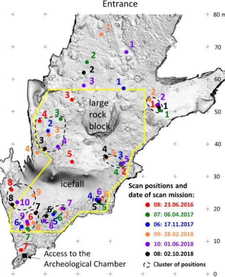
Figure 1.Location of the Silická l’adnica cave. The polygons represent the territory mapped by the TLS method – yellow outline delineates the area of scan mission 1 in 2016, and the red outline represents the area of other scan missions used to build a time series of TLS data. Contours and shaded relief improve the perception of numerous sinkholes on the plateau of Silická planina, which tend to have a regular funnel shape. The dark brown line denoted with “a” marks the vertical profile shown in Fig. 7. Numbered black crosshairs in a circle locate the ground control points used for registration into the common global coordinate system. Base maps: ©2019 GKÚ and ©2019 Esri.
Figure 2.Photographic evidence of cave floor ice in the Silická l’adnica cave over the last 80 years. All three photos are captured from approximately the same position (shown in Fig. 3 as a red point A) from inside the cave outward and show different states of cave floor ice. Identical points are marked in yellow. As a scale, objects marked in red can be used – (a) is the figure of a speleologist and (b) is a wooden stick 30 cm high. Based on the photographs we can conclude that there is a gradual loss of ice. The photographs were taken in different years but also at different periods within the year.
Sealed closing of the entrance into the chamber facilitates preservation of the static thermodynamic model of the cave (cold trap). Long-term monitoring revealed that the extent of the ice in the Silická l’adnica cave varies over short periods (Stankoviˇc and Horváth, 2004). The seasonal ice formations, which are the main source of water for new layers of floor ice, fill the cave in winter and grow until late spring, when they start degrading and re-icing at the lower, colder parts of the cave as floor ice. Permanent ice in the cave is kept only in the area of the icefall, which is replenished with new layers of ice during the summer, when it reaches its peak volume. The ice degrades during winter by sublimation and transfer of warm air from non-glaciated parts of the cave (Rajman et al., 1987).
3 Data and methods
Figure 3. Map of the Silická l’adnica cave floor. The cave is an open pit cave with the entrance being approximately 30 m wide and 20 m tall. It is freely accessible to the public from the north by a concrete staircase. Gravel and debris cover the floor mainly in the upper part of the cave near the entrance. There is a large limestone boulder labelled as a large rock block in the central part. The cave floor ice starts to occur from the boulder to the bottom part of the cave in the south. There are smaller blocks of rock in the ice and around the icefall. The deepest part of the Silická l’adnica cave is in the south. There is an artificial entrance to the Archaeological Chamber, which is closed by a hatch and covered with rock blocks. The red points and arrows mark the field of view in the photographs in Figs. 2 and 4.
The scanner rotates along its vertical axis establishing a full 360◦in the horizontal field of view. The vertical scan-ning angle is limited to 100◦. This means that from a single scanner position, it is not possible to capture a portion of the view under the scanner in the nadir direction and a part of the ceiling above the scanner in the zenith direction. The data shadows were eliminated by defining a proper configuration of positions during the scanning in which overlapping point clouds are generated.
The data collection by TLS in Silická l’adnica commenced in June 2016. The first campaign focused on testing the
capa-Figure 4. The Silická l’adnica cave contains different types of ice objects. The permanent ice is represented by (a) an icefall (Stankoviˇc and Horváth, 2004) located in the bottom part of the cave. Ice speleothems(b)such as stalactites and stalagmites situated in the upper part of the cave (Ondrej, 2014) are the most dynamic objects with significant seasonal and interannual changes. Approxi-mate size of the icefall can be judged based in the spelunker(s). The icefall is outlined with a white dashed line. The identical location of the ice stalactite in both photographs is marked for better orien-tation. White arrows indicate stalagmites (us – upper stalagmite; ls – lower stalagmite), which tend to accumulate in dry and wet sea-sons or years based on the size of the stalactite marked with a black arrow.
Figure 5.The workflow for generating a time series database and framework of data processing.
Figure 6.Distribution of scan positions of individual scan missions presented in the plan of the cave derived from TLS mapping. The yellow polygon shows a defined area of interest (AoI) for computa-tion of changes in ice accumulacomputa-tion.
time of scanning and achieving sufficient overlaps to elimi-nate shadows in the final point clouds (Fig. 6).
There were 32 individual scan positions used in the first mapping mission. The GCPs were placed in the close exte-rior of the cave; therefore several scan positions were also located in this area (Fig. 5 phase 1). The scan mission 1 used 10 GCPs for registration in global coordinate systems (Fig. 5 phase 4). Data from all scanning missions were registered in the national coordinate system S-JTSK (Systém jednotnej trigonometrickej siete katastrálnej), EPSG code 5514. The GCPs were measured by the global navigation satellite sys-tem (GNSS) using the Topcon HiPER II receiver with a refer-ence connection to the Slovak real-time positioning service – SKPOS. Point measurements were performed for 30 s using the real-time kinematic (RTK) positioning via weighted av-eraging with overall accuracy of the fixed solution between 1 and 2 cm. The coordinates of the points were calculated with Topcon Link software. The standard deviation error of trans-formation of scan mission 1 in the global coordinate system based on the GCPs was 5.3 cm.
The setting of scan parameters is reported differently by individual scanner manufacturers. We worked with 0.04 and 0.06◦ of angular increment in horizontal and vertical rota-tion, respectively. These modes are termed Panorama 40 and
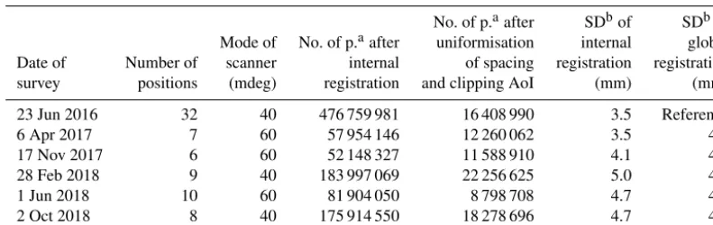
Panorama 60 in the Riegl VZ-1000 scanner. The increment defines the level of spatial detail captured by the scanner. The smaller the increment, the shorter the spacing between the recorded laser pulse echoes at the same range from the scan-ner. Table 1 summarises the generated datasets in terms of the amount of data and accuracy based on the scanning pa-rameters.
Precision of scan mission also depends on the number of scan positions. The largest point cloud was recorded within the first scan mission, where we scanned the surroundings of the cave. Subsequent scan missions were focused on acquir-ing data in the cave in places within the ice formation. There-fore, the number of scan positions and the number of points is lower in comparison with the first scan mission. Scanning at one position with scanner settings of range of 450 m, fre-quency of 300 kHz, and mode of Panorama 60 took almost 4 min while the duration of scanning was 5 min and 20 s with Panorama 40. The total scanning time of the first scan mis-sion was approximately 12 h due to the challenging terrain and the surrounding forest. Using selective a cloud-to-cloud (sC2C) approach enabled us to perform following scan mis-sions only inside the cave; thus scanning time did not exceed 3 h. Shorter time and fewer data are acceptable for repeating scanning to capture the ice accumulation dynamics and gen-eration of the time series database for long-term monitoring of cave cryomorphology. In the initial phase of the cave floor ice monitoring, we tested various parameters of the scanner settings. The aim was to find if a higher scanning detail in-fluences the precision of the mapping of cryomorphological topography. We found that critical points such as ice have the same point density even with higher scan detail. In addition, there are demands for processing and storing data because of their amount. During the 2-year mapping period, we also identified and optimised the scan positions, which we refer to as the scan position clusters (Fig. 6). Based on this testing, we learned that in our case a minimum of seven positions with Panorama 60 mode are sufficient to scan the cave floor ice.
3.1 A framework of registration procedure using TLS data
de-Table 1.Characteristics of the time series database.
No. of p.aafter SDbof SDbof
Mode of No. of p.aafter uniformisation internal global
Date of Number of scanner internal of spacing registration registration
survey positions (mdeg) registration and clipping AoI (mm) (mm)
23 Jun 2016 32 40 476 759 981 16 408 990 3.5 Reference
6 Apr 2017 7 60 57 954 146 12 260 062 3.5 4.4
17 Nov 2017 6 60 52 148 327 11 588 910 4.1 4.2
28 Feb 2018 9 40 183 997 069 22 256 625 5.0 4.2
1 Jun 2018 10 60 81 904 050 8 798 708 4.7 4.0
2 Oct 2018 8 40 175 914 550 18 278 696 4.7 4.5
aNo. of p. – number of points.bSD – standard deviation.
formation of the shape of the laser pulse trace. The scanner emits a laser pulse and distributes it to the ambient environ-ment. A laser pulse has a certain shape when it hits the sur-face. The scanner Riegl VZ-1000 is capable of recording the pulse deformation owing to the online waveform processing of the pulse. This parameter is termed deviation. It is a di-mensionless number with values from 0 to 65 535. The value 0 indicates that the track has a circular (ideal) shape, and the value 65 535 represents the shape of the elongated el-lipse of the pulse track. We kept only points with a devia-tion value between 0 and 20 as recommended by the scanner producer. Thus, we filtered out less accurate measurements caused by the deformed shape of the scanner pulse track. In addition, we used only points that represent the first and unique echoes. In this phase, we removed about 35 %–40 % of the points from the point clouds of single scan positions.
The next step was to calculate the normals for points (Fig. 5, phase 3). We recommend performing this step be-fore internal registration of mutual scan positions. The reason is that the direction of normals could be erroneously deter-mined for the cave after internal registration because of the complexity of cave geometry. Derivation of normals is re-quired for the generation of a 3-D model of the cave surface (Fig. 5, phase 8). The direction of the normals was calculated to the scanner position. In the case of irregular distribution of points it is more appropriate to calculate normal vectors with respect to the centre of each scan position than using algo-rithms based on neighbourhood analysis.
After filtering the points and calculating the normals, mutual orientation of the scan positions followed (Fig. 5, phase 4). It is termed the internal registration and it has two steps. First, the scans acquired within a single mission were coarsely registered via identical points identified in the area of the scans’ overlap. We chose edges of rocks on the ceiling and recognisable sharp objects, e.g. fault edges. The second step involved iterative closest point (ICP) adjustment, which is implemented in the RiSCAN Pro software as the Multi-Station Adjustment (MSA) module. The procedure uses the cloud-to-cloud approach to find the closest match of two or
more scans (Ullrich et al., 2003). This approach automati-cally searches and extract groups of points based on certain parameters. We used the method based on filtering planar patches. The minimum number of points to define a planar patch was set to five and the minimum search cube size was 0.128 m. Only the patches from which the points deviated by less than 0.02 m were used for registration of overlapping scans. Subsequently, centroids of the planes and the normals derived for them were determined. The registration of two scan positions is based on the assumption that the same ar-eas with the same or characteristics of normals very similar to the planar patches will be identified as identical within scenes being registered. The tolerance of the normals’ de-viation is defined by the parameter of maximum tilt angle, which was set to 1◦. Search radius was set to 0.5 m. Planar patches from two scans are considered identical if their cen-troids are within 0.5 m of each other (after coarse registration in the first step) and difference of the direction of their nor-mal at centroids does not exceed 1◦. Such a procedure was used to join all scans from a particular mission into a single point cloud located in a local coordinate system.
3.2 Selective cloud-to-cloud approach
The final point clouds from different missions required trans-formation into a common coordinate system to allow for the assessment of morphologic changes in ice accumulations. For this purpose, we designed an innovative sC2C approach to register scan missions into a unified coordinate system (Fig. 5, phase 4).
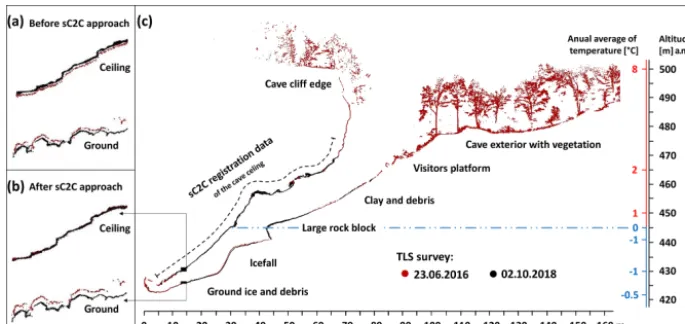
Figure 7.Demonstration of the improved registration accuracy by the sC2C method. Red dots represent the reference point cloud surveyed on 23 June 2016. The point cloud surveyed on 2 October 2018 marked with black dots was used to demonstrate the registration result using the proposed sC2C approach. The results of registering the two scan missions in the detailed views show the performance of(a)the standard C2C approach and(b)after applying the sC2C approach in which stable points of the cave ceiling(c)on the bare rock were used. The size of the cave can be estimated from the vertical and horizontal axes, which are in metres. The left side of the vertical axis shows mean annual air temperature inside the cave based on our temperature data loggers. The mean temperature is the lowest in the area of the icefall. The mean annual temperature of 0◦C is just above the icefall, indicating the approximate maximal vertical range of the cave floor ice.
of the plane centroids, which were determined according to the same parameters as in phase 4. We argue that for generat-ing a time series of point clouds, this kind of sC2C approach (Fig. 7b) based on cave ceiling performs better in the auto-matic registration of individual scan missions than a C2C ap-proach in which the entire scan is used for registration with another member of the time series (Fig. 7a). The point cloud of the reference scan mission was locked, and the propaga-tion of errors of identical planes was distributed only at loca-tions that we considered to be morphologically stable parts of the cave. By this means, in the registration of time series, we avoided the use of moving objects which did not change their geometry but changed their position or orientation, such as stones floating on the ice surface (Fig. 7a and b). Thus, the residuals of normals were not dispersed into places that could have been considered similar in shape but not identical in the position. Such an approach facilitates surface change detection. Finally, all final point clouds of individual mis-sions were placed in the S-JTSK global coordinate system to enable comparison with other older geodetic measurements. Laser scanning point clouds typically have heterogeneous spatial distribution of points. The first reason is in the very principle of data acquisition for which the point spacing in-creases with growing distance from the scanner; i.e. the point density per unit area decreases. Another reason is in the need of spatial overlap to perform the mutual registration of scans. The point density increases in the area of overlap, causing data redundancy in places that were in the scanner field of view from multiple positions. The marked variability in spa-tial distribution of the points within point clouds complicates interpolation of digital surface models and modelling derived surface parameters (Gallay et al., 2016). This complication
can be solved by making the distances between points more uniform (Fig. 5 phase 6). We used 0.005 m of spacing to dec-imate original point clouds, which reduced 60 % of points without a marked decrease in spatial detail captured in the final surface model. Homogenisation of the point distribu-tion was performed using the Octree tool implemented in the RiSCAN Pro software. By removing redundant points, we obtained a spatially homogenised input point cloud for the calculation of cave surface models.
The generated time series from point clouds representing the ice cave is another important outcome of the presented research (Fig. 5, phase 7) resulting from data collection and data processing (Fig. 5, phase 1 until phase 6).
3.3 Deriving complex 3-D cave model from point clouds using a mesh model
find a suitable surface. The result of the proposed modelling approach is still a 2-D surface (plate) which is located in 3-D space. Thus, the bivariate functions with the general form z=f (x, y)are not applied to the whole dataset in 2-D space. Instead, the 3-D space is fragmented locally into, for exam-ple, cubes with defined side lengths. This allows us to avoid conflicts in the computation ofzcoordinates. Therefore, we used a vector-based mesh modelling approach to create the surface of the cave floor, which makes it possible to model such complex shapes. One of the key inputs for calculation of mesh is vector normals of the points that have been derived in phase 3 for each scan position individually. We used the Poisson surface reconstruction (PSR) interpolation method (Kazhdan and Hoppe, 2013) implemented in the open-source software CloudCompare (Girardeau-Montaut, 2018). This global method using a B-spline was chosen because it com-bines the advantages of global and local surface reconstruc-tion methods without creating jagged polygons in phase of segments joining. Using the coordinates of input points in the form of control vector fields and normal vectors, PSR de-fines an indicator function to solve the Poisson equation at multiple octree levels resulting in derivation of iso-surfaces for individual fixed depths. Their values are used in the last step to reconstruct the resulting 3-D watertight surface. The generated cave surface model by PSR is dependent on sev-eral parameters. Spatial resolution of the 3-D cave surface model is controlled by the octree parameter. It is a dimen-sionless number used for fragmenting the space defined by the range of input data. Octree 1 means that the space of input data range is fragmented into eight cubes, which are identical to the bounding box cube of input data. Octree 2 means that each cube from the previous step is divided into eight smaller cubes. Thus, 64 smaller cubes are generated. In general, the resulting numbernof divisions of the input point cloud is calculated asn=8d, whered is the octree parame-ter (i.e. the octree depth). In our case, we used the value of Octree 13, whereby the whole space of input data range was fragmented to 813 (549, 755, 813, 888) cubes, which repre-sents a spatial resolution of 0.0054 m. The used octree value respected point spacing resolution of generated point clouds (Fig. 5, phase 6) without additional generalisation of the 3-D cave model. We used a high resolution of the octree param-eter because other paramparam-eters such as samples per node and point weight did not have a significant effect on the quality of the final 3-D cave models. For the so-called “full depth” pa-rameter, we set the value of 8, which represents a cube with an edge size of 0.1714 m. By this parameter, the spatial res-olution of triangles for parts of the 3-D cave model in places with a lower density of point distribution is set. The lower density of point distribution is located in the icefall, where the highest point-to-point distances reach 0.15 m. Thus, the parameter of the full depth helps us to regulate and limit cre-ation of longitudinal triangles.
After the 3-D cave model was created, it was necessary to cut the area of interest (AoI) (Fig. 5, phase 9). As the area of
interest we considered places on the floor of the cave, where we expect the occurrence of visible and buried floor ice. Sea-sonal ice coating on the walls and hanging from the ceiling was not included in the computation. We argue that all sea-sonal ice coating in the cave degraded and replenished cave floor ice. For better visualisation and understanding of ice dynamics, we have extended the polygon to the nearest sur-roundings. The AoI polygon projected orthogonally onto a plane defined byxandyaxes is 1200 m2. This step is neces-sary after 3-D cave modelling (Fig. 5, phase 8) because due to the interpolation function there is deformation in the model at the border of the AoI (border effect). We used a segment tool implemented in the CloudCompare software to cut the models based on the AoI polygon.
The resulting truncated 3-D floor cave models were sub-tracted from each other for calculating volumetric changes (Fig. 5, phase 10). To calculate volumetric changes, we used the M3C2 tool (Lague et al., 2013) implemented in the CloudCompare software. This tool uses normal vectors for computing the 3-D distances between two datasets. Differ-ences between 3-D floor cave models within the time se-ries database were expressed by cross sections and arrows representing movement of objects (Fig. 8), seasonal and an-nual changes via surfaces derived from the differences of dis-tances (DoDs) approach (Fig. 10), and numerically (Table 2).
4 Results and discussion
In this paper we introduce a new approach to generate time series by using TLS missions and the sC2C approach. This approach is characterised by the fact that no targets, mark-ers, or stabilised points are needed in the research area to place individual scan missions in a single coordinate system. As detailed in the methodology of this article, those parts of the cave that are stable are used to place the individual scan missions in a common coordinate system. In our case it is the ceiling of the cave. We decided to then analyse, us-ing two methods such as overlappus-ing cross sections (Fig. 8) and calculation of volumetric changes based on DoDs using 3-D floor cave models (Fig. 10) with interpretation, due to precipitation and temperatures during the monitored period (Fig. 9).
4.1 Detection of floor ice dynamics and analysis of its movements
er-ror and (2) the visual check on the overlapped vertical cross sections that represent point clouds from each scan mission.
The calculation of the standard deviation error of regis-tration was presented in Table 1. The internal regisregis-tration of scan positions within individual scan missions ranged from 3.5 to 5.0 mm. To compare the quality of internal registra-tion, we used the same parameters in the plane patch filter for all scan missions. We reached the lowest standard devia-tion error of internal registradevia-tion in the summer of 2016. This was because up to 24 positions were located in external parts around the cave, where the reflectivity of objects was higher, thus achieving better scanning quality. Although the number of scan positions was higher, the internal registration error was lower because the higher errors achieved in the cave at ice locations are masked by the lower errors achieved in the exterior parts of the cave; thus the overall standard deviation error is lower. This consideration can also be supported by the measurement on 6 April 2017, where there was a sig-nificant loss of ice. Thus, the reflectivity of the objects was higher, which resulted in a lower internal registration error. On the other hand, the highest internal registration error was achieved in the measurement in which new ice increments were recorded. It was a measurement from 20 February 2018. However, during all measurements, we achieved satisfactory results with internal registration. Using the sC2C approach, we have achieved an acceptable standard deviation of global registration, which ranges from 4.0 to 4.5 mm (Table 1).
The floor ice dynamics in the cave using the TLS method are captured with a degree of uncertainty, which is deter-mined by the device error (Einstrument)and the error of
regis-tering individual scan positions (Eregistration). One of
advan-tages of the proposed sC2C method is that there is no accu-mulation of errors due to errors in other measurements, such as GNSS (EGNSS)measurements and global coordinate
sys-tem registration error (EGCS). The total error (ETotal)of the
proposed method can be calculated using a modified Eq. (1) by Collins et al. (2012):
ETotal= q
E2instrument+Eregistration2 . (1) In our case, we used the Riegl VZ-1000 for mapping, whose Einstrumentis defined by the manufacturer and is 0.008 m. The
highest standard deviation error of global registration has been reached for the measurement on 2 October 2018 and has a value of 0.0045 m. The total errorETotalis±0.0092 m,
which is a threshold for recognising the changes between measurements. Thus, changes in point clouds of less than 0.0092 m cannot be interpreted as a change in the cave ice, as this may be an error propagation of the device and regis-tration.
We also evaluated the quality of registration of the scan missions in the common coordinate system by visual inspec-tion. The best way to evaluate registration quality is through visual inspection on profiles where the cloud points from each scan missions are rendered by a unique colour. During
the check we observe the course of point clouds and whether double surfaces of identical objects arise. In Fig. 7b it can be seen that the registration of scan missions by applying the sC2C approach achieves excellent ceiling performance, but there are larger variations on the floor of the cave. Based on a more detailed view of the cave floor presented in Fig. 8b, we conclude that the use of the sC2C approach is equally successful on the cave floor, except that the cave floor has changed in some places due to ice loss or accumulation. Ice dynamics is not the same in all locations. The biggest ice dynamics can be seen in the middle of the profile, which is related to the shape of the icefall.
The convergence of profile lines (areas where the lines be-come closer together) is not as observable as in the foot of the icefall (Fig. 8a) because there is a mechanically conditional movement of the material by spelunkers. In Fig. 8c, it is pos-sible to observe a random arrangement of the cross sections above a flat stone with a converging character. We argue that based on profile line analysis it is possible to detect area of ice occurrences in the cave. The locations of cross-section di-vergence (areas where the lines are farther apart) can be con-sidered to be the occurrences of cave floor ice, which may be covered by the sediment of a clastic unsorted material. This indicates the occurrences of buried ice.
A virtual tour of the cave as well as a visual inspection of the quality of registration of individual scan missions can also be performed through a Potree-based web application (Schuetz, 2016), which enables interactive work with scan point clouds of scan missions, for example creating verti-cal profiles in the optional direction, measurement of dis-tances, or changing number of rendered points. This web application contains a time series database, which will be continuously updated by newer scan missions aiming to doc-ument the cryomorphologic changes of the cave floor in the long-term perspective. The web-based interactive application is available at https://geografia.science.upjs.sk/webshared/ Laspublish/Ladnica/Silicka_ladnica_All.html (last access: 4 November 2019). For demonstration, we selected cross sec-tions passing through identical cave sites and across the cave floor. The line crosses different types of morphological struc-tures such as stone debris, icefall, subsurface floor ice, and stable elements such as large rocks attached to the subsoil structure (Fig. 8a).
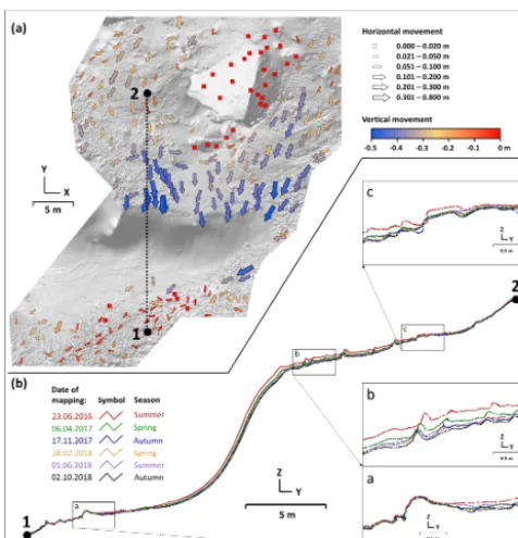
Figure 8. (a)Top view of the AoI-portraying cave floor model with the dotted line indicates the place of the vertical cross section. The arrows indicate the direction of ice movement. The size of the arrow reflects the length of movement in the horizontal direction and the colour expresses the length of movement in the vertical direction. Squares represent the places with no detected movement.(b)The overlaid cross sections represent the cave floor coloured by date of TLS mappings. Changes of the iced part of the cave floor are visu-alised in selected details. The details represent(a)the foot of the icefall,(b)the place of the most visible changes of the cave floor ice, and(c)the highest occurrence of floor ice in the cave in contact with stone debris.
the icefall or new ice accumulations bury them. If we look at the movement of ice in the horizontal plane, we can say that the floor ice seems to flow around a large stone block. How-ever, a number of factors need to be considered when inter-preting the movement of objects drowned in ice. The general tendency of the objects’ movement is in the direction of the lower parts of the cave. This suggests that one of the factors of movement is gravity. Objects from higher glaciated parts of the cave gradually move down. Furthermore, it is clear that the highest objects’ movement is near the icefall, where there is a significant horizontal and vertical movement. However, this movement is not the result of the movement of the ice-block itself, but the result of the loss of ice. This indicates that the ice is sublimating and melting at certain times of the year. This leads to a decrease in the volume of ice (Fig. 10) and thus the position of the objects changes as the volume of ice changes. Near the edge of the icefall there is the greatest thickness of ice, where during the monitored period the great-est losses of ice also occurred. In these places the movement of objects is the greatest. On the other hand, in places where the ice was able to recover, in the western part of the cave (to
the left of the large rock block) or where regular accumula-tions of ice occur by destruction of ceiling stalactites, there is less movement. In these places, the ice can recover. Another factor causing movement of objects is mechanical movement caused by spelunkers. This can be observed in particularly in the places where the path is (Fig. 3) and is reflected along the eastern edge (to the right of the large rock block) of the cave (Fig. 8). Analysis of movement of objects also suggests that the large rock block and the rocks below it are associated with the bedrock since they have changed by less than 2 cm during the reported period, which corresponds to the overall global registration error propagation.
4.2 Ice formation and ice dynamics
The results of the repeated terrestrial laser scanning based on the sC2C approach revealed changes of the ice surface and defined areal and volumetric changes. When evaluating and interpreting ice formation and dynamics of ice accumu-lations, it is necessary to support results with meteorological measurements of temperature and precipitation (Fig. 9). The meteorological data were recorded by the official meteoro-logical station in the Silica village located about 5 km east of the cave. The data on air temperature from the interior of the cave are from an automated data logger, which is located in Fig. 3.
The mean daily air temperature from the Silica weather station ranged from−15 to+28◦C throughout the monitored period. The highest temperatures were in summer, when the daily mean temperature did not drop below 12◦C. The lowest mean air temperatures occurred in winter, when their values oscillated around 0◦C and only sporadically rose above 5◦C. The monitored period was above the long-term average in comparison with the mean daily temperatures of the previous 30 years. Below-average daily temperatures occurred in two instances: autumn 2016 and the subsequent winter 2017 and winter 2018 during the winter–spring transition.
Figure 9.Long-term daily and monthly mean temperature (above the timeline) and precipitation (below the timeline) and their de-viations from the long-term average. The timeline shows the dates on which TLS mapping was performed. The background colours of the graph show the season (red – summer, yellow – autumn, blue – winter, green – spring). The bold dashed lines separate the years. Source: data supplied by SHMÚ (2019) and our own measurements.
renewed but the sublimation of the ice occurs. At the end of winter with the onset of spring, there is a transitional phase in which the greatest amount of ice is formed. The temperature of the cave is low after winter, but water in the surround-ing environment is in a liquid state and flows into the cave where it freezes. The onset of the summer phase of the cave occurs in the second half of spring, when the internal tem-perature of the cave gradually rises above 0◦C, mainly due to higher temperatures of the external environment and due to the penetration of warm water from precipitation into the cave. Thus, the formation and ablation of cave ice is influ-enced by precipitation, which is a source of water (Per¸soiu and Pazdur, 2011). The graph of monthly cumulative pre-cipitation (Fig. 9) indicates that the prepre-cipitation was mostly below average during the whole monitoring period. Precip-itation in June 2018 seems to be significantly above aver-age. However, there were only two precipitation events with short-term but intensive precipitation (summer storms). The situation was similar in July 2016.
For the formation of ice in the cave, the inflow of water into the cave during the transition phase (the end of winter and the first half of spring) is important. The rock and ice in the cave are cooled enough below 0◦C during this period.
If the inflow of water is sufficient, it has a significant effect on the increase in the amount of cave ice. Most of the ice mass in Silická l’adnica is found on the icefall. However, the recovery of ice on the icefall is gradual. The first stage in-volves formation of vertical ice stalactites (Fig. 4b). After melting, degradation, or collapse, the stalactites become the source of water for the formation of ice accumulations on the icefall. The equilibrium between the ice accumulation rate during different climate conditions is controlled by a com-plex interplay between the climatic factors that control the mass balance of ice, i.e. wet vs. dry summers and/or win-ters and cold vs. warm summers and/or winwin-ters (Per¸soiu and Pazdur, 2011). Ice increments in the Silická l’adnica occur mainly during the transition phase. During the summer and winter phases, there is a loss of ice. In the summer phase, the melting of ice is due to the higher temperature of the ambient air and warm water penetrating into the cave. Ice degradation in winter is mainly caused by ice sublimation. It is precisely this principle of ice formation and ablation in the Silická l’adnica that can be better described based on the time series of the TLS scan missions using DoD (Fig. 10 and Table 2). Seasonal comparison of surface dynamics (Fig. 10, seasonal) demonstrates that there is a constant change in ice volume (Table 2). Thus, the ice in the cave is constantly in-creasing or dein-creasing between time periods.
The biggest ice volume was recorded at the beginning of the monitoring in June 2016, as much water entered the cave due to above-average precipitation from the end of winter and early spring of 2016 (Fig. 9). Interestingly, the temper-ature in the cave at the turn of winter and spring 2016 was higher compared to the same period in spring 2017, but there was less ice in the cave (Figs. 9 and 10). A similar mete-orological situation was repeated at the turn of winter and spring 2018, although the amount of precipitation in this pe-riod was less than in spring 2016. Between summer 2016 and spring 2017 (Fig. 10, T1–T2) on icefall, while ice increment can be seen on a large stone block in the middle of the cave, where water dripping from vertical ice hanging from the ceil-ing formed ice accumulations (Fig. 4b). This phenomenon always occurs in the spring when the water from the melt-ing snow and sprmelt-ing rains passes through the cracks into the frozen part of the cave.
A similar phenomenon can be seen in Fig. 10 (T4–T5). Another phenomenon is the collapse of the glacial stalactites that we caught before the autumn (Fig. 10, T3–T4). Thus this phenomenon is not in the true sense of increments of cave ice volume, but the destruction of the original ice drops hanging from the ceiling. The ice degrades during the summer and autumn. In winter, a seasonal minimum in the volume of cave ice can be observed (Fig. 10, T2–T3 and T5–T6).
Figure 10.Differences of distances (DoD) between the individual cave floor surface models. Blue represents the decrease and red indi-cates the increase in the surface elevation. Arrows mark the position of the upper stalagmite (us) and lower stalagmite (ls).
of a dry spring the stalactite does not grow to a significant enough size to contribute with meltwater to the growth of the stalagmite right below it. When the stalactite is smaller, the dripping meltwater flows further down along the ceiling to another location and a new stalagmite accumulates just be-low the original one (Fig. 4a, white arrows). The change of volume of the ice stalagmites was recorded by monitoring with TLS. The lower stalagmite grew while the upper stalag-mite generally decreased during the whole surveying period (Fig. 10).
However, based on the presented analysis, we can con-clude that the assessment of floor cave ice dynamics in terms of overall trends is only possible to observe through a season-to-season comparison between the same periods, e.g. be-tween summer or spring seasons over a longer time period (Fig. 10, seasonal).
A considerable loss of ice formation volume has been seen in Fig. 10 (T1–T5), which demonstrates the rapid decrement
of ice between summer 2016 and summer 2018. DoD was calculated with respect to thezaxis, so there is a considerable drop in surface, even more than 2 m. However, it should be interpreted that if the ice on a steep icefall with a slope of more than 70◦falls 0.2 m in a direction perpendicular to the slope of the profile, the difference in zaxis (height) for a place with the samexandycoordinates can reach 2 m, which is visible from the comparison of individual cross sections (Fig. 8b and Table 2, max. decrease).
Red shows the increment in two places, which are demon-strated in Fig. 4. The increment in the massive rock in the middle of the cave was caused by the destruction of the glacial stalactite. The second distinctive height increment is located on the icefall in the form of a stalagmite, which is formed from dripping water from the shrinking stalac-tite hanging from the crevice in the cave ceiling, as de-scribed above. Another inter-seasonal comparison between spring 2017 and spring 2018 (Fig. 10, T2–T4) indicates a year-to-year loss of ice. In the case of DoD between au-tumn 2017 and auau-tumn 2018 (Fig. 10, T3–T6), there is no considerable decrement or increment of ice accumulations. We can conclude that the ice volume is comparable between these periods; so, it is relatively stable.
The biggest benefit of the created time series database of the complex 3-D surface model is also in the quantification of the volume changes of the cave floor ice and its expression through summary numerical statistics (Table 2).
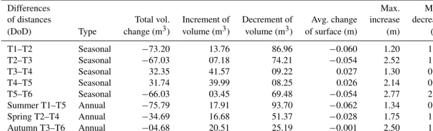
Given the total error ofETotal 0.0092 m and the area of
observation of 1200 m2, it should be emphasised that a vol-ume of up to 11.04 m3may be the result of a measurement error. The highest difference in ice volume was observed at the beginning of the monitored period between summer 2016 and spring 2017 (Fig. 10, T1–T2) and spring 2017 and au-tumn 2017 (Fig. 10, T2–T3), when a total ice loss was ap-proximately 70 m3in both cases (Table 2).
Considerable loss of ice in these periods can also be iden-tified from the average change of surface, which in this pe-riod reaches a loss of about 0.06 m. The highest increase was recorded between autumn 2017 and spring 2018, when new ice from spring rains is usually formed in the cave. The in-crease in ice should culminate in summer, but in 2018 there was little rainfall and it was relatively warm. The loss of ice between summer and autumn 2018 is already a natural phe-nomenon. The inter-seasonal comparison suggests that there is a considerable loss of ice due to the lack of water flow-ing into the cave durflow-ing the monitored period, as evidenced by the comparison between summer 2016 and summer 2018, when about 75 m3of ice was lost in the cave.
5 Conclusions
Table 2.Summary statistics of volumetric and vertical changes of the selected cave floor extent during the monitored period.
Differences Max. Max.
of distances Total vol. Increment of Decrement of Avg. change increase decrease
(DoD) Type change (m3) volume (m3) volume (m3) of surface (m) (m) (m)
T1–T2 Seasonal −73.20 13.76 86.96 −0.060 1.20 1.59
T2–T3 Seasonal −67.03 07.18 74.21 −0.054 2.52 1.38
T3–T4 Seasonal 32.35 41.57 09.22 0.027 1.30 0.96
T4–T5 Seasonal 31.74 39.99 08.25 0.026 2.14 0.89
T5–T6 Seasonal −66.03 03.45 69.48 −0.054 2.77 2.11
Summer T1–T5 Annual −75.79 17.91 93.70 −0.062 1.34 0.89
Spring T2–T4 Annual −34.69 16.68 51.37 −0.028 1.75 1.33
Autumn T3–T6 Annual −04.68 20.51 25.19 −0.001 2.50 1.33
recognisable because the caves are evidently linked with the immediate surroundings. The interpretation of the dynam-ics in the ice cave accumulations is a challenging task that should be based on long-term and regular monitoring. In this paper we presented the analysis of the floor ice dynamics in the Silická l’adnica cave.
Our research was inspired by the observations made from the middle of the 20th century, which reported ice formation and ablation in the Silická l’adnica cave (Roda et al., 1974; Rajman et al., 1987; Stankoviˇc and Horváth, 2004). The de-scribed thermodynamic regime and process of ice formations in Silická l’adnica are similar to the caves of Grotta del Gelo (Maggi et al., 2018), Ledenica u ˇCudinoj uvali (Buzjak et al., 2018), or Stojkova Ledenica (Neši´c and ´Cali´c, 2018), but most of these caves contain only seasonal ice formations. We also presented new results in the methodology of TLS data collection and processing, generation of a database of 3-D surface time series, floor ice dynamics evaluation using ob-ject movement analysis, and quantification of ice mass dy-namics based on complex 3-D cave models.
Terrestrial laser scanning was used to record the dynam-ics of cave sediments containing ice accumulations. In order to evaluate the changes in the cave ice accumulations, it was necessary to register the individual mappings into a uniform coordinate system. For this purpose, we proposed an innova-tive method based on automatic registration of the individ-ual scan positions using stable objects of the cave such as the ceiling of the cave. The presented sC2C approach reduces the overall registration error of the data time series into a unified coordinate system by avoiding the repeated positioning of GCPs by GNSS. We argue that the presented methodological framework of the sC2C approach has the potential to be used in other applications where it is necessary to identify land-scape dynamics, such as mountain glacier assessment and sediment accumulation dynamics analysis.
Finally, the developed methodological framework of data processing enables us to generate a 3-D time series database of the interior cave surface at ultra-high resolution. We also presented a procedure for the modelling of complex 3-D sur-faces from the point clouds. The presented data and methods
provided means for evaluating the dynamics of the cave floor ice. We detected the dynamics of the ice based on a cross-section method and via differences of 3-D distances analysis. Complex 3-D models of the cave floor were used to quantify the volumetric changes.
Results of the quantitative assessment of cryomorphologi-cal changes showed that there was a considerable loss of ice in the cave during the monitored period. The 3-D mapping over the 2-year period was coupled with continuous monitor-ing of air temperature inside and outside the cave and moni-toring of rainfall. Linking the findings on the dynamics of the cryomorphology and the meteorological monitoring shows the well-known fact that a cold but dry winter will lead to less ice accumulation compared to a warmer but wetter one, while a warm but dry summer will lead to less melting than a cold but wet one. Naturally, the question arises of whether there is irreversible year-to-year loss of ice mass or only a longer cycle of perennial ice accumulation replenishment. To be able to answer this question, it is necessary to continue monitoring cave ice and to analyse other factors such as tem-perature of precipitation, air circulation, evapotranspiration, tectonics and geological structure of the massif, morphology of the cave and immediate surroundings, and connection with other parts of the cave system.
Data availability. The time series database from the Silická l’adnica cave is available via the interactive web-based appli-cation: available at https://geografia.science.upjs.sk/webshared/ Laspublish/Ladnica/Silicka_ladnica_All.html (last access: 4 November 2019; šupinský, 2019).
reviewers; his role was important in the pre- and post-publication stages.
Competing interests. The authors declare that they have no conflict of interest.
Acknowledgements. The results achieved in the presented research originated thanks to the financial support by the grant of the Min-istry of Education, Science, Research and Sport of the Slovak Re-public within the projects VEGA 1/0963/17 “Landscape dynamics in high resolution” and VEGA 1/0839/18 “Development of a new v3.sun module designed for calculation of the solar energy distri-bution for digital geodata derived from a point cloud using adaptive triangulation methods” and by the Slovak Research and Develop-ment Agency for the financial support within the project APVV-15-0054: Physically based segmentation of geodata and its geoscience applications.
Financial support. This research has been supported by the Vedecká Grantová Agentúra MŠVVaŠ SR a SAV (grant nos. VEGA 1/0963/17 and VEGA 1/0839/18) and the Agentúra na Podporu Výskumu a Vývoja (grant no. APVV-15-0054).
Review statement. This paper was edited by Evgeny A. Podolskiy and reviewed by Aurel Per¸soiu, Manfred Buchroithner, and one anonymous referee.
References
Avian, M. and Bauer, A.: First results on monitoring glacier dynam-ics with the aid of Terrestrial Laser Scanning on Pasterze Glacier (Hohe Tauern, Austria), Grazer Schr. Geogr. Raumf., 41, 27–36, 2006.
Avian, M., Kellerer-Pirklbauer, A., and Lieb, G.: Geomorphic consequences of rapid deglaciation at Pasterze glacier, Hohe Tauern range, Austria, between 2010 and 2013 based on re-peated terrestrial laser scanning data, Geomorphology, 310, 1– 14, https://doi.org/10.1016/j.geomorph.2018.02.003, 2018. Barnhart, B. T. and Crosby, T. B.: Comparing Two Methods
of Surface Change Detection on an Evolving Thermokarst Using High-Temporal-Frequency Terrestrial Laser Scan-ning, Selawik River, Alaska, Remote Sens., 5, 2813–2837, https://doi.org/10.3390/rs5062813, 2013.
Bauer, A., Paar, G., and Kaufmann, V.: Terrestrial laser scanning for rock glacier monitoring, in: Permafrost, edited by: Phillips, M., Springman, S. M., and Arenson, L. U., Taylor and Francis, London, 55–60, 2003.
Bella, P.: Chapter 4.2 – Ice surface morphology, in: Ice Caves, edited by: Per¸soiu, A. and Lauritzen, S. E., Elsevier, 69–96, https://doi.org/10.1016/B978-0-12-811739-2.00029-2, 2018. Bella, P. and Zelinka, J.: Chapter 29 – Ice Caves in Slovakia, in:
Ice Caves, edited by: Per¸soiu, A., Lauritzen, S. E., Elsevier,
657–689, https://doi.org/10.1016/B978-0-12-811739-2.00029-2, 2018.
Bender, M., Sowers, T., and Brook, E.: Gases in ice
cores, P. Natl. Acad. Sci. USA, 94, 8343–8349,
https://doi.org/10.1073/pnas.94.16.8343, 1997.
Buchroithner, M. F., Milius, J., and Petters, C.: 3D Surveying and visualisation of the biggest ice Cave on Earth, in: Proceedings 25th International Cartographic Conference, Paris, France, 3–8 July 2011.
Buchroithner, M. F., Petters, C., and Pradhan, B.: Three-dimensional visualisation of the worldclass-prehistoric site of the Niah Great Cave, Borneo, Malaysia, in: Interdisciplinar Confer-ence on Digital Cultural Heritage, edited by: Kremens, H., Saint-Dié-des-Vosges, 2–4 July, 2012.
Buzjak, N., Boˇci´c, N., Paar, D., Bakši´c, D., and Duboveˇcak, V.: Chapter 16 – Ice Caves in Croatia, in: Ice Caves, edited by: Per¸soiu, A. and Lauritzen, S. E., Elsevier, 335–369, https://doi.org/10.1016/B978-0-12-811739-2.00016-4, 2018. Collins, B., Corbett, S., Fairly, H., Minasian, D., Kayen, R., Dealy,
T., and Bedford, D.: Topographic Change Detection at Select Archeological Sites in Grand Canyon National Park, Arizona, 2007–2010: US Geologic Survey Scientific Investigation Report 2012–5133, 77 pp., 2012.
Cosso, T., Ferrando, I., and Orlando, A.: Surveying and mapping a cave using 3D laser scanner: the open chal-lenge with free and open source software, Int. Arch. Pho-togramm. Remote Sens. Spatial Inf. Sci., XL-5, 181-186, https://doi.org/10.5194/isprsarchives-XL-5-181-2014, 2014. Deems, J., Painter, T., and Finnegan, D.: LiDAR
measure-ment of snow depth: a review, J. Glaciol., 215, 467–479, https://doi.org/10.3189/2013JoG12J154, 2013.
De Waele, J., Fabbri, S., Santagata, T., Chiarini, V., Columbu, A., and Pisani, L.: Geomorphological and speleogenetical observa-tions using terrestrial laser scanning and 3D photogrammetry in a gypsum cave (Emilia Romagna, N. Italy), Geomorphology, 319, 47–61, https://doi.org/10.1016/j.geomorph.2018.07.012, 2018. Droppa, A.: Gombasecká jaskyˇna [Gombasecká cave], Šport,
Bratislava, 115 pp., 1962.
Fabbri, S., Sauro, F., Santagata, T., Rossi, G., and De Waele, J.: High-resolution 3-D mapping using terrestrial laser scanning as a tool for geomorphological and speleoge-netical studies in caves: An example from the Lessini
mountains (North Italy), Geomorphology, 280, 16–29,
https://doi.org/10.1016/j.geomorph.2016.12.001, 2017. Faško, P. and Šˇtastný, P.: Mean annual precipitation totals, in:
Land-scape Atlas of the Slovak Republic, Ministry of Environment of the Slovak Republic, Bratislava/Slovak Environmental Agency, Banská Bystrica, Map No. 54, p. 99, 2002.
Fischer, M., Huss, M., Kummert, M., and Hoelzle, M.: Application and validation of long-range terrestrial laser scanning to monitor the mass balance of very small glaciers in the Swiss Alps, The Cryosphere, 10, 1279–1295, https://doi.org/10.5194/tc-10-1279-2016, 2016.
Fuhrmann, K.: Monitoring the disappearance of a perennial ice de-posit in Merrill Cave, J. Cave Karst Stud., 69, 256–265, 2007. Gabbud, C., Micheletti, N., and Lane, S. N.: Lidar
Gallay, M., Kaˇnuk, J., Hochmuth, Z., Meneely, J., Hofierka, J., and Sedlák, V.: Large-scale and high-resolution 3-D cave mapping by terrestrial laser scanning: a case study of the Domica Cave, Slovakia, Int. J. Speleol., 44, 277–291, https://doi.org/10.5038/1827-806X.44.3.6, 2015.
Gallay, M., Hochmuth, Z., Kanuk, J., and Hofierka, J.: Geomorpho-metric analysis of cave ceiling channels mapped with 3-D ter-restrial laser scanning, Hydrol. Earth Syst. Sci., 20, 1827–1849, https://doi.org/10.5194/hess-20-1827-2016, 2016.
Gašinec, J., Gašincová, S., ˇCernota, P., and Staˇnková, H.: Uses of Terrestrial Laser Sanning in Monitoring of Ground Ice within Dobšinská Ice Cave, J. Polish Mineral Eng. Soc., 30, 31–42, 2012.
Gašinec, J., Gašincová, S., Zelizˇnaková, V., Palková, J., and Kuze-viˇcová, Ž.: Analysis of Geodetic Network Established Inside the Dobšinská Ice Cave Space/Analýza Geodetickej Siete Zriadenej V Priestoroch Dobšinskej l’adovej Jaskyne, GeoScience Eng., 60, 45–54, https://doi.org/10.2478/gse-2014-0005, 2014. Girardeau-Montaut, D.: CloudCompare – 3D point cloud and mesh
processing software. Open Source Project, available at: https:// www.danielgm.net/cc/ (last access: 4 November 2019), 2018. Gómez-Lende, M. and Sánchez-Fernández, M.: Cryomorphological
Topographies in the Study of Ice Caves, Geosciences, 8, 250– 274, https://doi.org/10.3390/geosciences8080274, 2018. Gonzalez-Aguilera, D., Muoz, A. L., Lahoz, J. G., Herrero, J. S.,
Corchon, M. S., and Garcia, E.: Recording and modeling Pale-olithic caves through laser scanning, in: Proceedings of Inter-national Conference on Advanced Geographic Information Sys-tems & Web Services, Cancun, 19–26, 2009.
Hoffmeister, D., Zellmann, S., Kindermann, K., Pastoors, A., Lang, U., Bubenzer, O., Weniger, G. C., and Bareth, G.: Geoarchaeological site documentation and analysis of 3D data derived by terrestrial laser scanning, ISPRS Ann. Pho-togramm. Remote Sens. Spatial Inf. Sci., II-5, 173–179, https://doi.org/10.5194/isprsannals-II-5-173-2014, 2014. Idrees, M. O. and Pradhan, B.: 2016 – A decade of modern cave
surveying with terrestrial laser scanning: A review of sensors, method and application development, Int. J. Speleol., 45, 71–88, https://doi.org/10.5038/1827-806X.45.1.1923, 2016.
Jörg, P., Fromm, R., Sailer, R., and Schaffhauser, A.: Measuring snow depth with a terrestrial laser ranging system, in: Proceed-ings of the 2006 International Snow Science Workshop, Tel-luride, Colorado, 452–460, 2006.
Kaasalainen, S., Kaartinen, H., and Kukko, A.: Snow cover change detection with laser scanning range and brightness measure-ments, EARSeL eProceedings, 7, 133–141, 2008.
Kamintzis, J., Jones, P. P. J., Irvine-Fynn, T., Holt, O., Bunting, P., Jennings, S., Porter, P. R., and Hubbard, B.: Assessing the appli-cability of terrestrial laser scanning for mapping englacial con-duits, J. Glaciol., 243, 1–12, https://doi.org/10.1017/jog.2017.81, 2018.
Kazhdan, M. and Hoppe, H.: Screened Poisson
sur-face reconstruction, ACM Trans. Graph. 32, 29,
https://doi.org/10.1145/2487228.2487237, 2013.
Kern, Z: Chapter 5 – Dating Cave Ice Deposits in: Ice Caves, edited by: Per¸soiu, A. and Lauritzen, S. E., Elsevier, 109–122, https://doi.org/10.1016/B978-0-12-811739-2.00005-X, 2018.
Kern, Z. and Per¸soiu, A.: Cave ice – the imminent
loss of untapped mid-latitude cryospheric
palaeoen-vironmental archives, Quaternary Sci. Rev., 67, 1–7,
https://doi.org/10.1016/j.quascirev.2013.01.008, 2013.
Kern, Z. and Thomas, S.: Ice level changes from seasonal to decadal time-scales observed in lava tubes, lava beds national monument, NE California, USA, Geogr. Fis. Din. Quat., 37, 151–162, 2014. Kern, Z., Boˇci´c, N., and Sipos, G.: Radiocarbon-dated vegetal remains from the cave ice deposits of Velebit
mountain, Croatia, Radiocarbon, 60, 1391–1402,
https://doi.org/10.1017/RDC.2018.108, 2018.
Lague, D., Brodu, N., and Leroux, J.: Accurate 3D comparison of complex topography with terrestrial laser scanner: Application to the Rangitikei canyon (N-Z), ISPRS J. Photogramm., 82, 10-26, https://doi.org/10.1016/j.isprsjprs.2013.04.009, 2013.
Lapin, M., Faško, P., Melo, M., Šˇtastný, P., and Tomain, J.: Climatic regions, in: Landscape Atlas of the Slovak Republic, Ministry of Environment of the Slovak Republic, Bratislava/Slovak Environ-mental Agency, Banská Bystrica, map No. 27, p. 95, 2002. Lerma, L. J., Navarro, S., Cabrelles, M., and Villaverde, V.:
Ter-restrial laser scanning and close range photogrammetry for 3D archaeological documentation: the Upper Palaeolithic Cave of Parpalló as a case study, J. Archaeol. Sci., 37, 499–507, https://doi.org/10.1016/j.jas.2009.10.011, 2010.
Luetscher, M. and Jeannin, P.-Y.: A process-based classification of alpine ice caves, Theor. Appl. Karstology, 17, 5–10, 2004. Luetscher, M., Bolius, D., Schwikowski, M., Schotterer, U., and
Smart, P. L.: Comparison of techniques for dating of subsurface ice from Monlesi ice cave, Switzerland, J. Glaciol., 53, 374–384, https://doi.org/10.3189/002214307783258503, 2007.
Maggi, V. Colucci, R. R., Scoto, F., Giudice, G., and Ran-dazzo, L.: Chapter 19 – Ice Caves in Italy, in: Ice Caves, edited by: Per¸soiu, A., Lauritzen, S. E., Elsevier, 399–423, https://doi.org/10.1016/B978-0-12-811739-2.00019-X, 2018. Mavlyudov, B. R.: Chapter 4.1 – Ice Genesis and Types of Ice
Caves, in: Ice Caves edited by: Per¸soiu, A. and Lauritzen, S. E., 33–68, https://doi.org/10.1016/B978-0-12-811739-2.00032-2, 2018.
May, B., Spötl, C., Wagenbach, D., Dublyansky, Y., and Liebl, J.: First investigations of an ice core from Eisriesenwelt cave (Aus-tria), The Cryosphere, 5, 81–93, https://doi.org/10.5194/tc-5-81-2011, 2011.
Neši´c, D. and ´Cali´c, J.: Chapter 27 – Ice Caves in Serbia, in: Ice Caves, edited by: Per¸soiu, A. and Lauritzen, S. E., Elsevier, 611–624, https://doi.org/10.1016/B978-0-12-811739-2.00027-9, 2018.
Ondrej, Z.: Mikroklíma Silickej l’adnice a jej vplyv na zmeny l’adovej výplne [Microclimate of the Silická l’adnica cave and its influence on changes in ice filling], Diploma thesis, Univerzita P.J. Šafárika v Košiciach PF UPJŠ ÚGE, 91 pp., 2014.
Per¸soiu, A.: Chapter 4.3 – Ice Dynamics in Caves, in: Ice Caves, edited by: Per¸soiu, A. and Lauritzen, S. E., Elsevier, 97–108, https://doi.org/10.1016/B978-0-12-811739-2.00034-6, 2018. Per¸soiu, A. and Lauritzen, S. E.: Ice Caves, Elsevier, p. 752,
https://doi.org/10.1016/C2016-0-01961-7, 2018.
Per¸soiu, A. and Pazdur, A.: Ice genesis and its long-term mass balance and dynamics in Scarisoara Ice Cave, Romania, The Cryosphere, 5, 45–53, https://doi.org/10.5194/tc-5-45-2011, 2011.
Laser Radar Technology and Applications XIX; and Atmo-spheric Propagation XI (Vol. 9080, p. 90800J). International So-ciety for Optics and Photonics, 2014.
Pflitsch, A., Schörghofer, N., Smith, S. M., and Holmgren, D.: Mas-sive Ice Loss from the Mauna Loa Icecave, Hawaii, Arc. Antarc. Alpine Res., 48, 33–43, https://doi.org/10.1657/AAAR0014-095, 2016.
Prokop, A.: Assessing the applicability of terrestrial laser scanning for spatial snow depth measurements, Cold Reg. Sci. Technol., 54, 155–163, https://doi.org/10.1016/j.coldregions.2008.07.002, 2008.
Rajman, L., Roda, Š., Roda Jr., Š., and Šˇcuka, J.: Termodynamický režim Silickej l’adnice [Thermodynamic regime of the Silická l’adnica Cave], Slovenský kras, 25, 29–63, 1987.
Riegl Laser Measurement Systems GmbH, Austria: 3D Terrestrial laser scanner Riegl VZ-400/Riegl VZ-1000/Riegl VZ-2000 Gen-eral Description and Data Interfaces, 2015.
Roda, Š., Rajman, L., and Erdös, M.: Výskum mikroklímy a dy-namiky zal’adnenia v Silickej l’adnici [Research of microclimate and dynamics of the glaciation of Silická l’adnica Cave], Sloven-ský kras, 12, 157–174, 1974.
Rüther, H., Chazan, M., Schroeder, R., Neeser, R., Held, C., Walker, J. S., Matmon, A., and Horwitz, K. L.: Laser scanning for con-servation and research of African cultural heritage sites: the case study of Wonderwerk Cave, South Africa, J. Archaeol. Sci., 36, 1847–1856, https://doi.org/10.1016/j.jas.2009.04.012, 2009.
Schuetz, M.: Potree: Rendering Large PointClouds in Web Browsers. Diploma thesis, Vienna University of Technology, 92 pp., 2016.
SHMÚ: Slovenský hydrometeorologický úrad [Slovak hydrometeo-rological institute], Temperature and precipitation records for the Silica meteorological station from 05/2015 to 04/2019, 2019. Silvestre, I., Rodrigues, I. J., Figueiredo, M., and Veiga-Pires, C.:
High-resolution digital 3D models of Algar do Penico Cham-ber:limitations, challenges, and potential, Int. J. Speleol., 44, 25– 35, https://doi.org/10.5038/1827-806X.44.1.3, 2014.
Stankoviˇc, J. and Horváth, P.: Jaskyne Slovenského krasu v živote Viliama Rozložníka [Caves of the Slovak karst in live of Viliam Rozložnik], Speleoklub Minotaurus, Rožˇnava, 190 pp., 2004. Šupinský, J.: TLS time series of Silická l’adnica cave,
avail-able at: https://geografia.science.upjs.sk/webshared/Laspublish/ Ladnica/Silicka_ladnica_All.html, last access: 4 November 2019.
Ullrich, A., Schwarz, R., and Kager, H.: Using hybrid multi-station adjustment for an integrated camera laser-scanner system, Opti-cal 3-D Measurement Techniques IV, 1, 298–305, 2003. Vosselman, G. and Maas, H. G.: Airborne and terrestrial laser
scan-ning, Whittles Publishing, Dunbeath, p. 318, 2010.