Odds Generalized Exponential-Inverse Weibull Distribution: Properties & Estimation

(1)

Odds Generalized Exponential-Inverse Weibull Distribution:

Properties & Estimation

Amal Soliman Hassan

Mathematical Statistics, Cairo University

Institute of Statistical Studies and Research, Giza, Egypt [email protected]

Elsayed Ahmed Elsherpieny

Rokaya Elmorsy Mohamed

Abstract

Providing extended and generalized distribution is usually precious for many statisticians. A new distribution, called odds generalized exponential-inverse Weibull distribution (OGE-IW) is suggested for modeling lifetime data. Some structural properties of the new distribution are obtained. Three different estimation procedures, namely; maximum likelihood, percentiles and least squares, are used to estimate the model parameters of subject distribution. The consistency of the parameters of the OGE-IW distribution is demonstrated through a simulation study. A real data application is presented to illustrate the importance of the new distribution compared with some known distributions.

Keywords: T-X family, Inverse Weibull distribution; Maximum likelihood estimators; Least squares estimators, Percentiles estimators.

1. Introduction

(2)

function (pdf) and cumulative distribution function (cdf) of IW distribution with shape parameter and scale parameter  are given, respectively, by

1

( ; , ) x ; , 0, 0,

g x   x  e     x  (1)

( ; , ) x .

G x   e  (2)

Extended and generalized forms of IW distribution are studied by some authors, among them; Khan (2010) introduced and studied the beta inverse Weibull distribution. de Gusmão et al. (2011) introduced three-parameter inverse Weibull distribution, called the generalized inverse Weibull distribution, with unimodal, increasing and decreasing failure rates. Khan and King (2012) proposed four-parameter modified inverse Weibull distribution. Shahbaz et al. (2012) suggested the Kumaraswamy inverse Weibull distribution. Elbatal and Muhammed (2014) introduced the exponentiated generalized inverse Weibull distribution. The generalized inverse Weibull distribution including the exponentiated or proportional reverse hazard and Kumaraswamy generalized inverse Weibull distributions have been suggested by Oluyede and Yang (2014). Pararai et al. (2014) introduced gamma-inverse Weibull distribution based on gamma generated family. Khan et al. (2014) studied characterizations of the transmuted inverse Weibull distribution with an application to bladder cancer remission time's data. Khan and King (2016) introduced the four-parameter new generalized inverse Weibull distribution and investigated its potential usefulness with application to reliability data from engineering studies. Rodrigues et al. (2016) introduced exponentiated Kumaraswamy inverse Weibull distribution. Okasha et al. (2017) introduced the Marshall–Olkin extended inverse Weibull distribution.

The statistics literature is filled with lots of continuous univariate distributions for describing real data. In recent years, there has been a great interest among statisticians and applied researchers in constructing flexible distribution to facilitate better modeling of lifetime data in various situations. Several methods have been developed for generating new family of lifetime distributions. One approach of generalization was suggested by Marshall and Olkin (1997) by adding one parameter to the survival function

( ).

G x In the same trend, Gupta et al. (1998) added one parameter to the cdf G x( )of the baseline distribution to define the exponentiated–G class of distribution. Following Guptaʼs et al. class, Gupta and Kundu (1999) studied the two-parameter generalized exponential distribution as an extension of the exponential distribution. Our interest here with T-X family proposed by Alzaatreh et al. (2013), the cdf of T-X family is specified by

 

( ( )

 

0

, W G x

F x 



f t dt (3)

where, the random variable T called the transformer and W G x( ( ))be a function of ( ).

(3)

Alizadeh et al. (2017) proposed and studied a new generated family called the generalized odd generalized exponential.

Our motivation here is to introduce and study a new extended form for the inverse Weibull distribution with three parameters. We call the new distribution; the odds generalized exponential-inverse Weibull distribution, which is a particular case of T-X family of distributions. The rest of the paper contains the following sections. The new distribution is provided in Section 2. Some statistical properties are given in Section 3. Then, in Section 4, maximum likelihood, least squares and percentiles estimators are obtained. Simulation study and results are presented in Section 5. An application of the OGE-IW model to real data is presented in Section 6. At the end, concluding remarks are addressed in Section 7.

2. Construction of the OGE-IW Distribution

In this section, the pdf, cdf, reliabilty function, hazard rate function (hrf), reversed-hazard rate function and cumulative hazard rate function of OGE-IW distribution are derived. Expansions for its pdf and cdf are also provided.

We obtain the OGE-IW distribution by considering the exponential distribution as transformer in cdf (3); also, taking; W G x( ( ))G x

   

G x , the odds ratio of inverse Weibull distribution defined in (2) as follows





( )

1 ( ) ₁

0 0

; , , .

x x

e G x

G x _e

t t

F x e dt e dt

 

 

    

 









Hence, the cdf of OGE-IW distribution is as follows



; , ,



1 exp , 0

1 x

F x x

e 



   

 

  _ _



  

 (4)

The corresponding pdf is obtained as follows









2

1

; , , 1 exp .

1

x x

x

f x x e e

e

 



  





     

 

     

  _{ } _



  (5)

For 2, the OGE-IW reduces to a new model named as odds generalized exponential inverse Rayleigh distribuiton. For  1, OGE-IW reduces to another new model named as odds generalized exponential inverse exponential distribuiton.

(4)

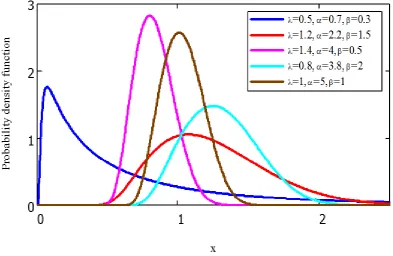
Figure 1: Plots of the pdf of OGE-IW distribution for selected values of the parameters

2.1 Expansion for Densities of OGE-IW Distribution

Two useful expansions of OGE-IW pdf and cdf are derived. Since, the pdf (5) can be rewritten as follows









2

1

; , , 1 exp .

1 x

x x

x

e

f x x e e

e



 

 

  



    



 

  

   



 

   _ _



  (6)

Then, by using the exponential expansion for the last term in (6) and further the binomial expansionfor a positive real power yields





 

1





1  1

, 0

2

; , , 1 .

! 2 !

j

j j i x

j i

j i

f x x e

j j i

 





     _{ } _ _{ } 



  

 

 



(7)

Then the pdf (7) can be formed as follows





, _ 1_

 

, 0

; , , _{j i} _{j i} ,

j i

f x    c g_ x



  





(8)

where, denotes the pdf of IW distribution g___{j i}_{ }₁_( )x and

 









1

,

1 1

! 2 !

j j j i

j i c

j j i

  _ _{ }

 

 

(5)

Further, an expansion for



F x( ; , , )  



t, for t a positive real power is derived as follows





, , _ _

 

0 , 0

( ; , , ) ,

t t

m l p l p m l p

F x     G_ x



  



 

(9)

where,

 



 



 

, , 1

! ! l m l t

m l p m

m l p

p l l



   

 

 and Glp

 

x is the cdf of IW with parameters



l p



and α.

2.2 Reliability Analysis

This subsection gives expressions for the reliability function, hazard function, and reversed hazard function.

The survival function and hrf of the OGE-IW distribution are respectively given by

( ; , , ) exp

1 x

F x

e 



   

 

 _{ } _



 ,





2

1

( ; , , ) 1 x .

h x    x  e  



  

 

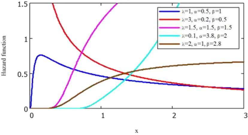
Figure 2 gives the plots of the hrf of OGE-IW distribution for some selected parameter values. Figure 2 indicates that OGE-IW hrfs can have increasing, decreasing and constant. This fact implies that the OGE-IW can be very useful for fitting data sets with various shapes.

(6)

The reversed-hazard rate function of the OGE-IW distribution is as follows





1 2 , , ( ; ) ,

1 exp 1

1 x x x x e x e e                           _ _ _ _     

Additionaly, the cumulative hazard rate function of the OGE-IW is given by



; , ,



ln exp

1 . x

H

e

x _ 

         _   _  

3. Some Mathematical Properties

In this section, some mathematical properties of the OGE-IW distribution, including, moments, probability weighted moments, incomplete moments, order statistics and entropy measure are derived.

3.1 Moments

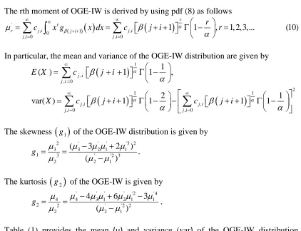
The rth moment of OGE-IW is derived by using pdf (8) as follows

 





, ₀ 1 ,

, 0 '

, 0

1 1 , 1, 2,3,... (10)

r r

j i j i j i

j i j

r

i

r

c x g_ x dx c j i  r

    _          _   _  _ _   







In particular, the mean and variance of the OGE-IW distribution are given by





1

, , 0

1

( ) _{j i} 1 1 ,

j i

E X c  j i 

      _   _  _ _  











2 1 1 , ,

, 0 , 0

2 1

var( ) _{j i} 1 1 _{j i} 1 1

j i j i

X c  j i  c  j i 

             _   _  _ __ _   _  _ __   _  _



The skewness

 

g₁ of the OGE-IW distribution is given by

' ' '

2 3 2

3 3 2 1 1

1 3 ' ' 2 2 '2 3 1

3 2 )

. ) (

(

g    



 

  

 



The kurtosis

 

g₂ of the OGE-IW is given by

2 4

4 3 1 2 1 1

4

2 2 2 2

2

' ' ' ' ' '

' '

2 1

4 6 3

( )

g      

          .

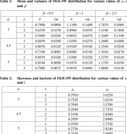
Table (1) provides the mean (μ) and variance (var) of the OGE-IW distribution for various parameter values. From Table (1), we notice that both values of the mean and variance of the OGE-IW decrease as the values of  and_{increases. Also, the values of} the mean and variance increase as the values of _{increase. Table (2) contains the} skewness and kurtosis of the OGE-IW distribution for various values of parameters and

.We notice that both the skewness and the kurtosis are decreasing functions of and .

(7)

Table 1: Mean and variance of OGE-IW distribution for various values of  ,

and 

0.5

   1  2.5

   var  var  var

2

1 0.7900 0.0800 1.1180 0.1600 1.7670 0.4000 2 0.6330 0.0370 0.8960 0.0470 1.4160 0.1840 3 0.5660 0.0240 0.8010 0.0470 1.2660 0.1180

4.5

1 0.8870 0.0200 1.0350 0.0270 1.2680 0.0400 2 0.8070 0.0120 0.9420 0.0160 1.1540 0.0240 3 0.7700 0.0085 0.8980 0.0740 1.1010 0.0170

5

1 0.8970 0.0160 1.0300 0.0220 1.2370 0.0310 2 0.8240 0.0098 0.9470 0.0130 1.1370 0.0190 3 0.7900 0.0072 0.9070 0.0096 1.0890 0.0140

Table 2: Skewness and kurtosis of OGE-IW distribution for various values of  and

  g₁ g₂

2

1 0.7910 3.6220

2 0.7530 3.6210

3 0.7040 3.5700

4.5

1 0.2940 2.7570

2 0.3100 2.8560

3 0.2950 2.8980

5

1 0.2550 2.7230

2 0.2750 2.8240

3 0.2630 2.8690

Furthermore, the moment generating function of OGE-IW can be obtained as follows

 

,





0 0 , 0

1 1

, 1, 2,...

! !

r r

x j i

r r j i

r

t j i

t

M t E X c r

r r

 



  

  

 

   

  _ _

  _ _







 



3.2 Probability Weighted Moments (PWMs)

Greenwood et al. (1979) introduced the probability weighted moments to derive estimators of the parameters and quantiles of distributions. The PWMs of OGE-IW distribution is defined by

 





 

,t ,

t _r

r

t r

E X F x x F x f x dx

 



(8)

where, t and r are positive integers. Inserting pdf (8) and cdf (9) in (11), then the PWMs of the OGE-IW distribution is obtained as follows









, , , ,

1 0 , , , 0

1 1

. 1 t

r t m l p j i r

m l p j i

r j i

c

j i p l 

              _ _           

 

3.3 Incomplete Moments

Theis defined by £_s

 

a , moment, sayincomplete sth

 

£ s ( ) .

a

s a x f x dx 





(12)

Hence, the sth moment of OGE-IW is derived by inserting (8) in (12) as follows

 









, 0

, 1 1 1 .

£ ,

s

j i

s j i

s

c j i j i a

a    

            _  _  



(13)

where, 1 s ,



j i 1



a 





 

 _   _

  is the upper incomplete gamma function. In particular,

the first incomplete moments of the OGE-IW distribution can be obtained by puttings 1 in (13), as follows

 





1





, 0

1 ,

1

1 1 , 1 .

£

j i j i

c j i j i a

a    

            _  _  



(14)

Bonferroni and Lorenz curves are useful applications to first incomplete moments. These curves are very useful in economics, reliability, demography, insurance and medicine. The Lorenz and Bonferroni curves are obtained, respectively, as follows













1 , 0 1 , , , 0 0 1

1 1 , 1

, 1 1 1 1 ( ) ( ) ( ) j i j i j i j i x F

c j i j i x

c j

L x af a

i da E X                   _   _           _ _   _ _  





and













1 , 0 1 , , , 0 1

1 1 , 1

( )

( ) = .

( ) 1

1 exp 1 1

1 j i j i F F j i x j i

c j i j i x

L x B x

F x

c j i

e          _             _   _     _ _  _ _{ } _ _{ }       _ _ _   _ _  



Another application of the first incomplete moments refers to the mean deviations which provide useful information about the characteristics of a population. Indeed, the amount of dispersion in a population may be measured to some extent by the totality of the deviations from the mean and median. The mean deviations of X about the meanand  about the median

m

can be calculated from the following relations

1 2 F( ) 2 ( )T and 2 2 ( ),T m

(9)

where,

0 ( ) ( )

q

T q 



xf x dx which is the first incomplete moment, then from (14)

( ) and ( )

T  T m are obtained, respectively, as follows





1





, , 0 0

1

( ) ( ) _{j i} 1 1 , 1 ,

j i

T xf x dx c j i j i

                  _   _  









1





, 0 , 0

1

( ) ( ) _{j i} 1 1 , 1 .

m

j i

T m xf x dx c  j i   j i m 

           _   _  





3.4 Rényi Entropy

The entropy of a random variable X with density function f x( ) is a measure of the uncertainty variation. The Rényi entropy is defined as

1

( ) ( ) ,

1 R

I  ln f  x dx 

 

 

 _ _

 _



_ (15)

where  0_and  1. Applying the exponential and binomial expansions, then ( ; , , )

f  x    can be expressed as follows

   

 1





 





 2 

0

2

( ; , , ) 1 1 (16)

! 2 !

j i x j j

j

j _x

j

x j i e

f x e

j j i

        _  _{  }                           



Inserting (16) in (15), then the Rényi entropy of OGE-IW distribution becomes

 







 



 





1 1 1 , 0

2 1 1

1 ! 1 ( ! ) 2 . 1 j j j j i R j i

j i j

I l i n j  _ _                               _ _     _         _ _  _ _   



3.5 Order Statistics

Let X_1:_n  X_2:_n  ... X_{n n}_: denote the order statistics for a random sampleX X₁, ₁,...,X_n from OGE-IW distribution with pdf (8) and cdf (9). The pdf of rth order statistics is defined by

 





 





1

:

0 1

1 ( ) ( ) .

, 1 n r k r k r n k n r

f x F x f x

k B r n r

 _{ }





 

 _ _ 

 



_ _ (17)

Using the binomial expansion for



F x( )



k r 1, replacing t in (9) withk  r 1. Hence the pdf (17) becomes

 





1 1  1

: , , , , ,

0 0 , , , 0 1

, (18)

, 1

n r k r

j i l p x

r n k j i m l p

k m j i l p

f x x e

B r n r

                     

  

where

 

1



  

  



, , , , ,

1

2

1

.

2

! ! ! !

l j

k j m l

k j i m l p

n r

k

r

j

i

m

p l

k

m

j

l j i l p







  







 





  

 

 







  

(10)

In particular, the pdf of the smallest order statistics is obtained by substituting r 1 in (18) as follows

 

1 1 1  1

1: , , , , ,

0 0 , , , 0

, n k r

j i l p x

n k j i m l p

k m j i l p

f x n  x  e  

              

  

where

 

1



  



 



, , , , ,

1 2

1 .

2 ! ! ! ! l

j m l _j

k j i m l p

n k j i m p l

k m j l j i l p



       _     

  _ _{ }

  

  

Also, the pdf of largest order statistics is obtained by substituting rn in (18) as follows

 

1

1 1

:

0 , ,

, , , 0

, , ,

( ) ,

k r

j i l p x n n

m j i l p

k j i m l p

f x n  x  e  

            

 

where

 

1



  



 



, , , , ,

1 2

1 .

2 ! ! ! ! l

j m l j

k j i m l p

k n j i m p l

m j l j i l p



       _     

  _ _

  

 

4. Parameter Estimation

In this section, the parameter estimators of the OGE-IW model parameters are obtained based on maximum likelihood (ML), least squares (LS) and percentiles methods.

4.1 Maximum Likelihood Estimators

In this subsection, the estimation of the unknown parameters of the OGE-IW distribution is considered using the ML method. Let X₁,...,X_n be observed values from the OGE-IW distribution. The total log-likelihood function, denoted bylnL, for the parameters , and  in complete sample is as follows









1 1 1 1

ln n ln nln n ln 1 ln 2 ln 1 .

1

i i

n n n n

x

i i _x

i i i i

L x x e

e                             _ _    



The partial derivatives of the log-likelihood function with respect to , and  componentsof the score vector U_L (U U U_, _, _)T can be obtained as follows

1

ln

1

,

i n i x

L

n

U

e

 



_  





 























2





1 1 1 1

ln ln

ln

ln ln 2 ,

1 1 i i i i x x

n n n n

i i i i

i i i _x

x

i i i i

n x x e x x e

L

x x x

e e U            _ _    _                    



_ 



_





2





1 1 1

ln

1

2

.

1

i i i

n n n

i i

i

i i i

x

x x

x

e

x

(11)

Then the maximum likelihood estimates (MLEs) of the parameters, denoted byˆ,ˆ and ˆ

 are obtained by setting U U_, _ and U_ to be zero and solving them numerically.

4.2. Least Squares Estimator

Suppose that X X₁, ₂,...,X_n is a random sample of sizen from the OGE-IW distribution and suppose X_1:_n X_2:_n  ... X_{n n}_: denotes the corresponding ordered sample. The LS estimators of the unknown parameters , and  denoted by  %%, and % of the OGE-IW distribution can be obtained by minimizing the sum of squares errors with respect to

,

  and,

2

1

: ( )

1 . i

n n i

i F x

n



 

  

  



So the LS estimators  %%, and %of the OGE-IW model can be obtained by minimizing the following quantity

2

1

1 exp ,

1 1

i

n

x i

i n e 

  

 

 

 _ _ 

 

 _ _ _ 

   



with respect to , and respectively.

4.3. Percentiles Estimator

Let X X₁, ₂,...,X_nbe a random sample from the OGE-IW, let X_{i n}_: denotes the ith order statistic, i.e, X_1:_n X_2:_n  ... X_{n n}_: . If p_i denotes some estimates ofF x



_{i n}_: ; , ,  



, then the estimator of unknown parameters, denoted by , and , can be obtained by minimizing the following equation with respect to, and 

 

2

1

1 exp

ln l .

1 n

i

n

x i

i

e

p _ 

  

    

 

  _  

 

  



 





In percentiles method (PM) of estimate, p_i takes a several possible choice as estimates forF x



_{i n}_: ; , ,  



, in this study, the formula

1 i

i p

n



 , is the expected value of the

OGE-IW distribution and will be used.

5. Numerical Study

In this section, numerical study is performed to evaluate and compare the performance of the estimates with respect to their biases, and mean square errors (MSEs) for different

sample sizes and for different parameter values. The numerical procedures are described

(12)

Step(1): A random sampleX₁,...,X_n of sizes n=(10,20,30,50,100) are selected, these random samples are generated from the OGE-IW distribution by using the following transformation





1 1

, 1, 2,... 1

1 ,

i

ln

ln u

x i n



 



  _ 



 _ 

 



  

 

  and ui are random sample from uniform(0,1).

Step(2): Eightdifferent set values of the parameters are selected as, ( =0.2, =0.5, =0.1), ( =0.2, =0.5, =0.3), (

1 2 3 =0.2, =0.5, =0.5),

set     set     set    

( =0.2, =0.5, =0.7), ( =0.2, =0.75, =0.3)

4 5 , 6 ( =0.2, =1, =0.3),

set     set     set    

( =0.2, =1.25, =

7 0.3)

set     and set8( =0.2, =1.5, = 3   0. ).

Step(3): For each model parameters and for each sample size, the MLEs, LS estimates and percentiles estimates (PEs) of λ,α and β arecomputed.

Step(4): Steps from 1 to 3 are repeated 1000 times for each sample size and for selected sets of parameters. Then, the biases and MSEs of the estimates of the unknown parameters are computed.

Numerical results are reported in Tables (3) to (6) and represented through some Figures from (3) to (6). From these tables, the following conclusions can be observed on the properties of estimated parameters from the OGE-IW distribution.

1- The biases of  in the percentiles method decrease as the value of  increases. Also, the biases of  increase as the value of  increases, for different set of parameters,in approximately all sets of parameters.

2- The biases and MSEs of MLEs, forandare smaller than the corresponding for .

3- For fixed values of, and as the values of increase, the biases and MSEs are decreasing, in approximately most of situations (see Table 4). As the values of  increase and for fixed values ofMSEs for all , the biases and and  estimates decrease in approximately, most sample sizes (see Table 5).

4- The biases and MSEs of ML estimates, forand are smaller than the corresponding for.

(13)

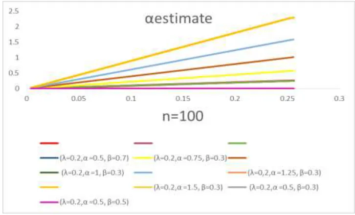
Figure 3: MSE for MLE for the set 2

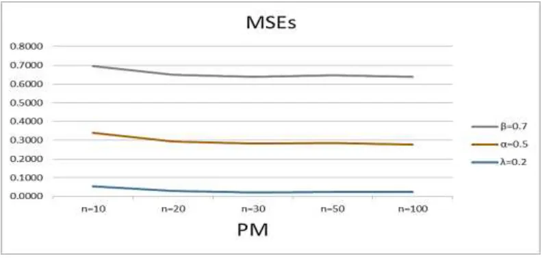
Figure 4: MSE for PE for the set 4

6- The MSEs for the LS estimates,% and %take the smallest value among the corresponding MSEs for the other methods in almost all of the cases (see Tables (3) and (4)).

7- The biases of  in the PM decrease as the value of  increases. Also, the biases of  increase as the value of  increases, for different set of parameters, in approximately all sets of parameters.

(14)

Figure 5: MSEs ofˆ, %and for all set of parameters

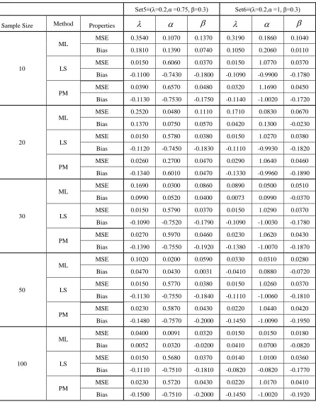
9- For fixed values of, and as the values of increase, the biases and MSEs are decreasing, in approximately most of situations (see Table 4). As the values of  increase and for fixed values ofMSEs for all , the biases and and  estimates decrease in approximately, most sample sizes (see Table 5).

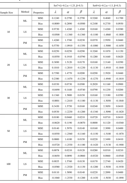
10- As it seems from Figure (6),the MSEs of the MLEs of _{take the smallest values} corresponding to the other estimates %and  for the same sample size. Also the MSEs of for all sets of parameters have the smallest values for the same sample size. The set 6 of parameters gives the smallest MSEs for different estimates corresponding to other set of parameters.

(15)

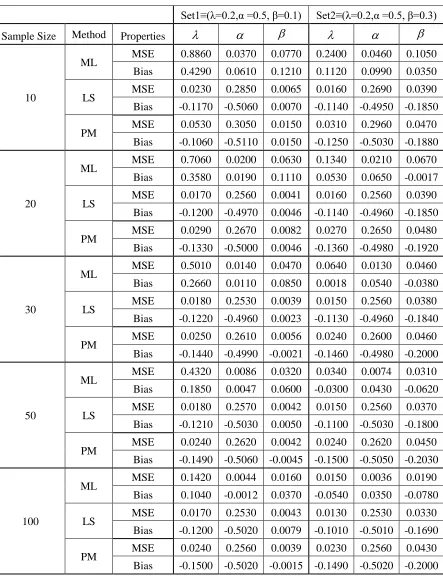
Table 3: Biases and MSEs of estimates for set1and set2, for the Odds Generalized Exponential Inverse Weibull distribution

Set1≡(λ=0.2,α =0.5, β=0.1) Set2≡(λ=0.2,α =0.5, β=0.3)

Sample Size Method Properties      

10

ML MSE 0.8860 0.0370 0.0770 0.2400 0.0460 0.1050 Bias 0.4290 0.0610 0.1210 0.1120 0.0990 0.0350 LS MSE 0.0230 0.2850 0.0065 0.0160 0.2690 0.0390 Bias -0.1170 -0.5060 0.0070 -0.1140 -0.4950 -0.1850 PM MSE 0.0530 0.3050 0.0150 0.0310 0.2960 0.0470 Bias -0.1060 -0.5110 0.0150 -0.1250 -0.5030 -0.1880

20

ML MSE 0.7060 0.0200 0.0630 0.1340 0.0210 0.0670 Bias 0.3580 0.0190 0.1110 0.0530 0.0650 -0.0017 LS MSE 0.0170 0.2560 0.0041 0.0160 0.2560 0.0390 Bias -0.1200 -0.4970 0.0046 -0.1140 -0.4960 -0.1850 PM MSE 0.0290 0.2670 0.0082 0.0270 0.2650 0.0480 Bias -0.1330 -0.5000 0.0046 -0.1360 -0.4980 -0.1920

30

ML MSE 0.5010 0.0140 0.0470 0.0640 0.0130 0.0460 Bias 0.2660 0.0110 0.0850 0.0018 0.0540 -0.0380 LS MSE 0.0180 0.2530 0.0039 0.0150 0.2560 0.0380 Bias -0.1220 -0.4960 0.0023 -0.1130 -0.4960 -0.1840 PM MSE 0.0250 0.2610 0.0056 0.0240 0.2600 0.0460 Bias -0.1440 -0.4990 -0.0021 -0.1460 -0.4980 -0.2000

50

ML MSE 0.4320 0.0086 0.0320 0.0340 0.0074 0.0310 Bias 0.1850 0.0047 0.0600 -0.0300 0.0430 -0.0620 LS MSE 0.0180 0.2570 0.0042 0.0150 0.2560 0.0370 Bias -0.1210 -0.5030 0.0050 -0.1100 -0.5030 -0.1800 PM MSE 0.0240 0.2620 0.0042 0.0240 0.2620 0.0450 Bias -0.1490 -0.5060 -0.0045 -0.1500 -0.5050 -0.2030

100

(16)

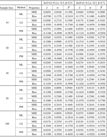
Table 4: Biases and MSEs of estimates for set3and set4, for the Odds Generalized Exponential Inverse Weibull distribution

Set3≡(λ=0.2,α =0.5, β=0.5) Set4≡(λ=0.2,α =0.5, β=0.7)

10

ML MSE 0.0650 0.0540 0.1300 0.0460 0.0560 0.2800 Bias -0.0780 0.1370 -0.2410 -0.1370 0.1480 -0.4850 LS MSE 0.0200 0.2710 0.1500 0.0170 0.2660 0.3420 Bias -0.1050 -0.4950 -0.3760 -0.1060 -0.4930 -0.5800 PM MSE 0.0750 0.2890 0.1600 0.0550 0.2840 0.3570

Bias -0.1180 -0.4990 -0.3870 -0.1110 -0.4950 -0.5830

20

Bias -0.1380 -0.4960 -0.3940 -0.1290 -0.4950 -0.5850

30

Bias -0.1450 -0.4970 -0.3990 -0.1420 -0.4970 -0.5950

50

Bias -0.1500 -0.5050 -0.4040 -0.1470 -0.5040 -0.6000

100

(17)

Table 5: Biases and MSEs of estimates for set5and set6, for the Odds Generalized Exponential Inverse Weibull distribution

Set5≡(λ=0.2,α =0.75, β=0.3) Set6≡(λ=0.2,α =1, β=0.3)

10

ML

MSE 0.3540 0.1070 0.1370 0.3190 0.1860 0.1040

Bias 0.1810 0.1390 0.0740 0.1050 0.2060 0.0110

LS

MSE 0.0150 0.6060 0.0370 0.0150 1.0770 0.0370

Bias -0.1100 -0.7430 -0.1800 -0.1090 -0.9900 -0.1780

PM

MSE 0.0390 0.6570 0.0480 0.0320 1.1690 0.0450

Bias -0.1130 -0.7530 -0.1750 -0.1140 -1.0020 -0.1720

20

ML

MSE 0.2520 0.0480 0.1110 0.1710 0.0830 0.0670

Bias 0.1370 0.0750 0.0570 0.0420 0.1300 -0.0230

LS

MSE 0.0150 0.5780 0.0380 0.0150 1.0270 0.0380

Bias -0.1120 -0.7450 -0.1830 -0.1110 -0.9930 -0.1820

PM

MSE 0.0260 0.2700 0.0470 0.0290 1.0640 0.0460

Bias -0.1340 0.6010 0.0470 -0.1330 -0.9960 -0.1890

30

ML

MSE 0.1690 0.0300 0.0860 0.0890 0.0500 0.0510

Bias 0.0990 0.0520 0.0400 0.0073 0.0990 -0.0370

LS

MSE 0.0150 0.5790 0.0370 0.0150 1.0290 0.0370

Bias -0.1090 -0.7520 -0.1790 -0.1090 -1.0030 -0.1780

PM

MSE 0.0270 0.5970 0.0460 0.0230 1.0620 0.0430

Bias -0.1390 -0.7550 -0.1920 -0.1380 -1.0070 -0.1870

50

ML

MSE 0.1020 0.0200 0.0590 0.0330 0.0310 0.0280

Bias 0.0470 0.0430 0.0031 -0.0410 0.0880 -0.0720

LS

MSE 0.0150 0.5770 0.0380 0.0150 1.0260 0.0370

Bias -0.1130 -0.7550 -0.1840 -0.1110 -1.0060 -0.1810

PM

MSE 0.0230 0.5870 0.0430 0.0220 1.0440 0.0420

Bias -0.1480 -0.7570 -0.2000 -0.1450 -1.0090 -0.1950

100

ML

MSE 0.0400 0.0091 0.0320 0.0150 0.0150 0.0180

Bias 0.0052 0.0320 -0.0200 0.0410 0.0700 -0.0820

LS

MSE 0.0150 0.5680 0.0370 0.0140 1.0100 0.0360

Bias -0.1110 -0.7510 -0.1810 -0.0820 -0.0820 -0.1770

PM

MSE 0.0230 0.5720 0.0430 0.0220 1.0170 0.0410

(18)

Table 6: Biases and MSEs of estimates for set7and set8, for the Odds Generalized Exponential Inverse Weibull distribution

Set7≡(λ=0.2,α =1.25, β=0.3) Set8≡(λ=0.2,α =1.5, β=0.3)

10

ML

MSE 0.1240 0.2790 0.2790 0.5260 0.4040 0.1700

Bias -0.0089 0.2890 -0.0500 0.2100 0.2730 0.0930

LS

MSE 0.9730 1.4260 1.4260 0.0160 2.4260 0.0380

Bias -0.0500 -1.1360 -0.1360 -0.1100 -1.4860 -0.1800

PM

MSE 1.4260 1.3760 0.0230 0.0370 2.5950 0.0460

Bias 0.5750 -1.0910 -0.1350 -0.1080 -1.5000 -0.1650

20

ML

MSE 0.0250 0.0250 0.0290 0.3260 0.1870 0.1150

Bias -0.0550 0.1910 -0.0790 0.1280 0.1640 0.0420

LS

MSE 0.3690 1.5120 0.0170 0.0160 2.3140 0.0390

Bias 0.1010 -1.2010 -0.1230 -0.1130 -1.4910 -0.1840

PM

MSE 0.7390 1.4770 0.0200 0.0290 2.3920 0.0460

Bias 0.2380 -1.1670 -0.1230 -0.1270 -1.4940 -0.1810

30

ML

MSE 0.0330 0.0730 0.0300 0.2020 0.1160 0.0900

Bias -0.0490 0.1440 -0.0740 0.0790 0.1230 0.0200

LS

MSE 0.1360 1.5800 0.0150 0.0160 2.3180 0.0390

Bias -0.0001 -1.2410 -0.1180 -0.1130 -1.5050 -0.1840

PM

MSE 0.3430 1.5750 0.0160 0.0240 2.3850 0.0410

Bias 0.0530 -1.2230 -0.1200 -0.1340 -1.5090 -0.1820

50

ML

MSE 0.0180 0.0460 0.0210 0.0720 0.0710 0.0410

Bias -0.0620 0.1190 -0.0870 0.0000 0.1120 -0.0360

LS

MSE 0.0140 1.5970 0.0140 0.0160 2.3090 0.0400

Bias -0.0550 -1.2560 -0.1160 -0.1150 -1.5100 -0.1870

PM

MSE 0.0800 1.6100 0.0150 0.0220 2.3490 0.0410

Bias -0.0720 -1.2530 -0.1180 -0.1420 -1.5130 -0.1900

100

ML

MSE 0.0078 0.0210 0.0120 0.0280 0.0310 0.0210

Bias -0.0650 0.0890 -0.0860 -0.0320 0.0860 -0.0540

LS

MSE 0.0035 1.5760 0.0130 0.0170 2.2740 0.0420

Bias -0.0580 -1.2520 -0.1130 -0.1200 -1.5030 -0.1930

PM

MSE 0.0110 1.5890 0.0140 0.0220 2.2890 0.0400

(19)

6. Data Analysis

In this section, we provide a data analysis in order to assess the goodness-of-fit of the OGE-IW model comparing with some known distributions such as the exponential (E) generalized exponential (GE) generalized inverse Weibull (GIW), Kumaraswamy inverse Weibull (KIW), Marshpall–Olkin extended inverse Weibull (MOEIW) and IW. The data set refers to Lee and Wang (2003) which represent remission times (in months) of a random sample of 128 bladder cancer patients. The data are as follows:

0.08 2.09 3.48 4.87 6.94 8.66 13.11 23.63 0.2 2.23 0.52 4.98 6.97 9.02 13.29 0.4 2.26 3.57 5.06 7.09 0.22 13.8 25.74 0.5 2.46 3.46 5.09 7.26 9.47 14.24 0.82 0.51 2.54 3.7 5.17 7.28 9.74 14.76 26.31 0.81 0.62 3.28 5.32 7.32 10.06 14.77 32.15 2.64 3.88 5.32 0.39 10.34 14.38 34.26 0.9 2.69 4.18 5.34 7.59 10.66 0.96 36.66 1.05 2.69 4.23 5.41 7.62 10.75 16.62 43.01 0.19 2.75 4.26 5.41 7.63 17.12 46.12 1.26 2.83 4.33 0.66 11.25 17.14 79.05 1.35 2.87 5.62 7.87 11.64 17.36 0.4 3.02 4.34 5.71 7.93 11.79 18.1 1.46 4.4 5.85 0.26 11.98 19.13 1.76 3.25 4.5 6.25 8.37 12.02 2.02 0.31 4.51 6.54 8.53 12.03 20.28 2.02 3.36 6.76 12.07 0.73 2.07 3.36 6.39 8.65 12.63 22.69 5.49 .

Measures of fit statistic using the maximized log-likelihood



2 logL



, Akaike information criterion



AIC



, the corrected Akaike information criterion



CAIC



, and Hannan-Quinn information criterion



HQIC



,are provided in Table 7. The model with minimum values for 2logLor AIC or BIC or CAICor HQIC can be chosen as the best model to fit the data. The ML estimates and their standard errors (SE) for OGE-IW, GE, E, GIW, KIW, MOEIW and IW models are given in Table 8.

Table 7: The statistics2logL ,AIC , CAIC , BIC and , HQIC , for the 128 bladder cancer patients data

Distribution ‐2logL AIC BIC CAIC HQIC

OGE-IW 801.263 807.263 807.585 807.457 810.740

GE 805.022 809.022 809.236 809.118 811.339

E 827.296 829.296 829.403 829.328 830.455

GIW 874.450 880.450 863.673 880.644 883.926

KIW 971.574 979.574 980.003 979.899 984.209

MOEIW 810.707 816.707 817.029 816.901 820.183

(20)

Table 8: ML estimates of the model parameters and the corresponding SEs for the 128 bladder cancer patient's data

Distribution ˆ ˆ



ˆ

_aˆ _bˆ _ˆ_

OGE-IW 0.057

(0.05)

0.87 (0.076)

0.336 (0.244)

- -

GE 0.111

(0.013)

0.922 (0.107)

- -

E 0.075

(0.008)

- -

GIW 0.75

(0.25)

0.53 (0.038)

1.797 (0.324)

- -

KIW -

-

3.796 (0.238)

2.239 (2.846)

0.0077 (0.006)

0.093 (0.012)

- -

MOEIW -

-

0.047 (0.049)

1.39 (0.104)

- -

198.304 (221.399)

IW 16.142

(0.125)

0.464 (0.042)

- -

The results show that the OGE-IW distribution provides a significantly better fit than the other models.

7. Conclusion

In this article, we propose a new model, called the odds generalized exponential-inverse Weibull distribution based on T-X family presented by Alzaatreh et al. (2013). Some statistical properties of current distribution are derived and discussed. The estimation of the model parameters is approached by maximum likelihood, least squares and percentiles methods. Simulation study is carried out to compare the performance of different estimates. Simulation study revealed that the PEs perform well than the MLEs and LS estimates, in approximately, most of situations. An application to a real data set indicates that the new model is superior to the fits than the other well-known distributions.

References

1. Alizadeh, M., Ghosh, I., Yousof, H. M., Rasekhi, M., and Hamedani, G. G. (2017). The generalized odd generalized exponential family of distributions: Properties, characterizations and application. Journal of Data Science, 15(3), 443-465.

(21)

3. Calabria, R., and Pulcini, G. (1990). On the maximum likelihood and least squares estimation in the inverse Weibull distribution, Statistica Applicata, 2, 53-66.

4. Calabria, R., and Pulcini, G. (1994). Bayes two-sample prediction for the inverse Weibull distribution. Communications in Statistics—Theory & Methods, 23, 1811-1824.

5. de Gusmão, F. R. S., Ortega, E. M. M., and Cordeiro, G. M. (2011). The generalized inverse Weibull distribution. Statistical Papers, 52, 591–619.

6. Elbatal, I., and Muhammed, H. Z. (2014). Exponentiated generalized inverse Weibull distribution. Applied Mathematical Sciences, 8, 3997-4012.

7. Greenwood, J. A., Landwehr, J. M. and Matalas, N. C. (1979) probability weighted moments: Definitions and relations of parameters of several distributions expressible in inverse form. Water Resources Research, 15, 1049-1054.

8. Gupta, R. D., and Kundu, D. (1999). Generalized exponential distribution. Australian and New Zealand Journal of Statistics, 41 (2), 173–188.

9. Gupta, R. C, Gupta, P. I. and Gupta, R. D. (1998). Modeling failure time data by Lehmann alternatives. Communications in Statistics-Theory and Methods, 27, 887–904.

10.Hassan, A. S., and Al-Thobety, A. K. (2012). Optimal design of failure step stress partially accelerated life tests with type II inverted Weibull data. International Journal of Engineering Research and Applications, 2(3), 3242-3253.

11.Hassan, A. S., Assar, M. S., and Zaky, A. N. (2015)) constant-stress partially accelerated life tests with type II inverted Weibull distribution with multiple censored data. International Journal of Advanced Statistics and Probability, 3(1), 72-82.

12.Keller, A. Z., and Kamath, A. R. (1982). Reliability analysis of CNC machine

tools. Reliability engineering, 3, 449–473.

13.Khan, M. S. (2010). The beta inverse Weibull distribution. International Transactions in Mathematical Sciences and Computer, 3,113–119.

14.Khan, M. S., and King, R. (2012). Modified inverse Weibull distribution. Journal of Statistics Applications & Probability, 1, 115–132.

15.Khan, M. S., and King, R. (2016). New generalized inverse Weibull distribution for lifetime modeling. Communications for Statistical Applications and Methods, 23(2), 147–161

16.Khan, M. S., King, R., and Hudson, I. L. (2014). Characterizations of the transmuted inverse Weibull distribution, ANZIAM Journal, 55, 197–217.

17.Lee, E. T., and Wang J. W. (2003). Statistical Methods for Survival Data Analysis. 3rd edition, Wiley, New York, http://dx.doi.org/10.1002/0471458546. 18.Maiti, S. S., and Pramanik, S. (2015). Odds generalized exponential-exponential

(22)

19.Marshall, A.W and Olkin, I. (1997). A new method for adding a parameter to a family of distributions with applications to the exponential and Weibull families. Biometrika, 84, 641–652.

20.Okasha, H. M., El-Baz, A.H., Tarabia, A. M. K., Basheer, A. M. (2017). Extended inverse Weibull distribution with reliability application. Journal of the Egyptian Mathematical Society, 25, 343-349.

21.Oluyede, B. O., and Yang, T. (2014). Generalizations of the inverse Weibull and related distributions with applications. Electronic Journal of Applied Statistical Analysis, 7(1), 94-116.

22.Pararai, M., Warahena-Liyanage, G., and Oluyede, B.O. (2014). A new class of generalized inverse Weibull distribution with applications. Journal of Applied Mathematics & Bioinformatics, 4(2), 17-35.

23. Rodrigues, J. A., Silva, A. P. C. M., and Hamedani, G. G. (2016). The exponentiated Kumaraswamy inverse Weibull distribution with application in survival analysis. Journal of Statistical Theory and Applications, 15(1), 8-24. 24.Shahbaz, M. Q., Shahbaz, S. and Butt, N. S. (2012). The Kumaraswamy–

inverse Weibull distribution. Pakistan Journal of Statistics and Operation

Research, 8(3), 479-489.