www.clim-past.net/12/1079/2016/ doi:10.5194/cp-12-1079-2016
© Author(s) 2016. CC Attribution 3.0 License.
A Late Pleistocene sea level stack
Rachel M. Spratt and Lorraine E. Lisiecki
Department of Earth Science, University of California, Santa Barbara, California, USA
Correspondence to: Lorraine E. Lisiecki ([email protected])
Received: 7 July 2015 – Published in Clim. Past Discuss.: 13 August 2015
Revised: 26 February 2016 – Accepted: 18 March 2016 – Published: 26 April 2016
Abstract.Late Pleistocene sea level has been reconstructed from ocean sediment core data using a wide variety of prox-ies and models. However, the accuracy of individual recon-structions is limited by measurement error, local variations in salinity and temperature, and assumptions particular to each technique. Here we present a sea level stack (average) which increases the signal-to-noise ratio of individual reconstruc-tions. Specifically, we perform principal component analysis (PCA) on seven records from 0 to 430 ka and five records from 0 to 798 ka. The first principal component, which we use as the stack, describes ∼80 % of the variance in the data and is similar using either five or seven records. After scaling the stack based on Holocene and Last Glacial Max-imum (LGM) sea level estimates, the stack agrees to within 5 m with isostatically adjusted coral sea level estimates for Marine Isotope Stages 5e and 11 (125 and 400 ka, respec-tively). Bootstrapping and random sampling yield mean un-certainty estimates of 9–12 m (1σ) for the scaled stack. Sea level change accounts for about 45 % of the total orbital-band variance in benthic δ18O, compared to a 65 % contri-bution during the LGM-to-Holocene transition. Additionally, the second and third principal components of our analyses re-flect differences between proxy records associated with spa-tial variations in theδ18O of seawater.
1 Introduction
Glacial–interglacial cycles of the Late Pleistocene (0–800 ka) produced sea level changes of approximately 130 m, pri-marily associated with the growth and retreat of continen-tal ice sheets in 100 ka cycles. Recent ice sheet modeling studies support the assertion of Milankovitch theory that Late Pleistocene glacial cycles are primarily driven by insolation changes associated with Earth’s orbital cycles (Ganopolski
and Calov, 2011; Abe-Ouchi et al., 2013). However, model-ing ice sheet responses over orbital timescales remains quite challenging, and the output of such models should be eval-uated using precise and accurate reconstructions of sea level change. Thus, Late Pleistocene sea level reconstructions are important both for understanding the mechanisms responsi-ble for 100 ka glacial cycles and for quantifying the ampli-tude and rate of ice sheet responses to climate change. Sea level estimates for warm interglacials at 125 and 400 ka are also of particular interest as potential analogs for future sea level rise (Kopp et al., 2009; Raymo and Mitrovica, 2012; Dutton et al., 2015).
Nearly continuous coral elevation data have generated well-constrained sea level reconstructions since the Last Glacial Maximum (LGM) at 21 ka (Clark et al., 2009; Lam-beck et al., 2014). However, beyond the LGM sea level es-timates from corals are discontinuous and have relatively large age uncertainties (e.g., Thompson and Goldstein, 2005; Medina-Elizalde, 2013). Several techniques have been devel-oped to generate longer continuous sea level reconstructions from marine sediment core data. Each of these techniques is subject to different assumptions and regional influences. Here, we identify the common signal present in seven Late Pleistocene sea level records as well as some of their differ-ences.
These sediment core records convert δ18Oc, the
oxy-gen isotope content of the calcite tests of foraminifera, to sea level using one of several techniques. In three records, temperature proxies were used to remove the temperature-dependent fractionation effect fromδ18Ocin order to solve
for the δ18O of seawater (δ18Osw). Other techniques for
transformingδ18Oc to sea level include the polynomial
re-gression of δ18Oc to coral-based sea level estimates,
tech-niques produce slightly different results for a variety of rea-sons. For example,δ18Oswvaries spatially due to differences
in water mass salinity and deep water formation processes (Adkins et al., 2002). Reconstructions also vary based on sensitivity to eustatic versus relative sea level (RSL) and tem-poral resolution.
Principal component analysis (PCA) is used to identify the common sea level signal in these seven records (i.e., to pro-duce a sea level “stack”) and to evaluate differences between reconstruction techniques. By combining multiple sea level records with different underlying assumptions and sources of noise, the sea level stack should have a higher signal-to-noise ratio than the individual sea level records used to construct it. We estimate the uncertainty of the sea level stack using bootstrapping and Monte Carlo-style random sampling. For comparison, we also report the standard deviation of high-stand and lowhigh-stand estimates across individual records and the sea level uncertainties of individual records as estimated in their original publications. A probabilistic reassessment of the uncertainties in individual records is beyond the scope of the current study.
2 Sea level reconstruction techniques
2.1 Corals and other coastal sea level proxies
Corals provide the most prominent Late Pleistocene sea level proxy. They can be radiometrically dated and provide es-pecially accurate sea level estimates between 0 and 21 ka because of nearly continuous pristine coral specimens from several locations (Fairbanks, 1989; Bard et al., 1990, 1996; Edwards et al., 1993). Dated coral sea level estimates ex-tend as far back as∼600 ka (Stein et al., 1993; Stirling et al., 1995; Medina-Elizalde, 2013; Muhs et al., 2014; Ander-sen et al., 2008). However, coral data are increasingly dis-continuous and inaccurate prior to 21 ka due to difficulty finding pristine and in situ older corals (particularly during sea level lowstands) and due to U–Th age uncertainties in older corals caused by isotope free exchange with the sur-rounding environment (e.g., Thompson and Goldstein, 2005; Blanchon et al., 2009; Medina-Elizalde, 2013). Interpreta-tion of sea level from corals often requires a correcInterpreta-tion for rates of continental uplift, which may not be known pre-cisely (Creveling et al., 2015). Glacial isostatic adjustment (GIA) and species habitat depth (up to 6 m below sea level) may also affect sea level estimates (Raymo and Mitrovica, 2012; Medina-Elizalde, 2013). Wave destruction and climate variations also alter coral growth patterns and may affect the height of colonies relative to sea level (Blanchon et al., 2009; Medina-Elizalde, 2013).
Organic proxies such as peat bogs and shell beds can also be used as sea level proxies and can be radiometrically dated (e.g., Horton, 2006). Geological formations indicating sea level such as abandoned beaches and sea cliffs can also be
used as sea level proxies (Hanebuth et al., 2000; Boak and Turner, 2005; Bowen, 2010).
Corals and other coastal proxies are indicators of relative (local) sea level and, thus, are affected by in situ glacio-isostatic effects, ocean siphoning processes, and other local effects of sea level rise and fall. However, their wide spa-tial distribution, particularly corals in tropical regions, allows for modeling of glacio-isostatic adjustments (GIA) to create a global estimate of mean sea level change (e.g., Kopp et al., 2009; Lambeck et al., 2014; Dutton and Lambeck, 2012; Hay et al., 2014). GIA models constrained by these coastal indicators provide robust sea level change estimates of−130 to −134 m for the LGM (Clark et al., 2009; Lambeck et al., 2014). A compilation of dozens of corals and other sea level indicators also provide relatively well-constrained es-timate of 8.7±0.7 m for peak global mean sea level at the last interglacial (Kopp et al., 2009). Estimates from multiple studies using different data are all in relatively good agree-ment yielding a consensus estimate of 6–9 m above mod-ern (Dutton et al., 2015). Additionally, sea level during last interglacial likely experienced several meters of millennial-scale variability (Kopp et al., 2013; Govin et al., 2012). Uncertainties increase for older interglacials. GIA-corrected coastal sea level proxies for Marine Isotope Stage (MIS) 11 at∼400 ka suggest a global mean sea level of 6–13 m above modern (Raymo and Mitrovica, 2012).
2.2 Seawaterδ18O
Global ice volume is a main control on the global mean of δ18O in seawater (δ18Osw), with global mean δ18Osw
estimated to decrease by 0.008–0.01 ‰ m−1 of sea level rise (Adkins et al., 2002; Elderfield et al., 2012; Shakun et al., 2015). However, δ18Osw also varies spatially based
on patterns of evaporation and precipitation and deep wa-ter formation processes. Theδ18O of calcite (δ18Oc) is
af-fected both by theδ18Oswand temperature. In the absence of
any post-depositional alteration, subtracting the temperature-dependent fractionation effect from δ18Oc (Shackleton,
1974) should yield a good estimate of theδ18Oswin which
the calcite formed. Pioneering studies for estimating time se-ries ofδ18Osw using independent measures of temperature
include Dwyer et al. (1995), Martin et al. (2002), and Lea et al. (2002). Dwyer et al. (1995) used ostracod Mg/Ca ratios to determine temperature whereas Martin et al. (2002) and Lea et al. (2002) used benthic and planktonic foraminifera, respectively. Theδ18Oc of benthic foraminifera reflects the
temperature andδ18Osw of deep water, while the δ18Oc of
planktonic foraminifera is affected by sea surface tempera-ture (SST) and theδ18Oswof near-surface water.
2.3 Benthicδ18Osw
Our analysis includes two benthicδ18Oswrecords from the
ra-tio of benthic foraminifera as a temperature proxy. The South Pacific benthic δ18Oswrecord (Elderfield et al., 2012) from
Ocean Drilling Program (ODP) site 1123 (171◦W, 41◦S;
3290 m) reflects the properties of Lower Circumpolar Deep Water, which is a mix of Antarctic Bottom Water (AABW) and North Atlantic Deep Water (NADW). Mg/Ca ratios and
δ18Oc were determined from separate samples of the same
species of Uvigerina, which is considered fairly insensitive to the deep water carbonate saturation state (Elderfield et al., 2012). Elderfield et al. (2012) interpolate their data to 1 ka spacing, perform a 5 ka Gaussian smoothing, and convert fromδ18Oswto sea level using a factor of 0.01 ‰ m−1.
Elder-field et al. (2012) report measurement uncertainties for tem-perature andδ18Ocgenerate aδ18Oswuncertainty of±0.2 ‰,
corresponding to bottom water temperature range of±1◦C or about 22 m of sea level.
The North Atlantic δ18Osw reconstruction is from Deep
Sea Drilling Program (DSDP) site 607 (32◦W, 41◦N;
3427 m) and nearby piston core Chain 82-24-23PC (Sosdian and Rosenthal, 2009). These sites are bathed by NADW to-day but were likely influenced by AABW during glacial max-ima (Raymo et al., 1990). Mg/Ca was measured using two benthic foraminiferal species, Cibicidoides wuellerstorfi and
Oridorsalis umbonatus, which may be affected by changes
in carbonate ion saturation state, particularly when deep wa-ter temperature drops below 3◦C (Sosdian and Rosenthal, 2009). Theδ18Ocdata come from a combination of Cibici-doides and Uvigerina species. Sea level was estimated from
benthicδ18Oswusing a conversion of 0.01 ‰ m−1and then
taking a three-point running mean. Combining the uncer-tainties for temperature (±1.1◦C) and δ18O
c (±0.2 ‰)
re-ported by Sosdian and Rosenthal (2009) yields a sea level uncertainty of approximately ±20 m (1 standard error) for the three-point running mean.
2.4 Planktonicδ18Osw
A 49-core global stack uses the δ18Oc from planktonic
foraminifera paired with SST proxies from the same core. The planktonic species in this reconstruction were G.
ru-ber, G. bulloides, G. inflata, G. sacculifer, N. dutretriei,
and N. pachyderma. Forty-four records span the most recent glacial cycle, and seven records extend back to 798 ka. Thirty-four records use Mg/Ca temperature esti-mates, and 15 use the alkenone Uk370 temperature proxy. Be-cause Uk370 measurements derive from coccolithophore rather than foraminifera, there is some chance the temperature mea-sured may differ slightly from that affectingδ18Oc(Schiebel
et al., 2004). However, Shakun et al. (2015) observed no sig-nificant differences in δ18Osw estimated from the two SST
proxies. An additional concern is that the surface ocean is affected by greater hydrologic variability and characterizes a smaller ocean volume than the deep ocean. Thus, plank-tonicδ18Oswmay differ more from ice volume changes than
benthic data. However, these potential disadvantages of
us-ing planktonic records may be largely compensated by the use of a global planktonic stack.
The first principal component (stack) of the planktonic records spanning the last glacial cycle represents 71 % of the variance in the records (n=44), suggesting a strong common signal in planktonicδ18Osw. However, the 800 ka
planktonicδ18Oswstack appears to contain linear trends that
differ from other sea level estimates. Therefore, Shakun et al. (2015) corrected their sea level estimate by detrending planktonicδ18Oswbased on differences between planktonic
and benthicδ18Oc. Standard errors reported by Shakun et
al. (2015) for theδ18Oswstack increase from 0.05 ‰ for the
last glacial cycle to 0.12 ‰ at 800 ka due to the reduction in the number of records. The equivalent sea level uncertainties are±6 and±18 m (1σ), respectively. All data were interpo-lated to even 3 ka time intervals.
2.5 Benthicδ18Oc– coral regression
The sea level reconstruction of Waelbroeck et al. (2002) was developed by fitting polynomial regressions between ben-thicδ18Oc from North Atlantic cores NA 87-22/25 (55◦N,
15◦W; 2161 and 2320 m) and equatorial Pacific core V19-30 (3◦S, 83◦W; 3091 m) to sea level estimates for the last glacial cycle, primarily from corals. Quadratic polynomials were fit during times of ice sheet growth and during the glacial termination in the North Atlantic whereas a linear re-gression was fit to the Pacific glacial termination. A compos-ite sea level curve was created from the most reliable sections of several cores, primarily from the Pacific. Waelbroeck et al. (2002) interpolated the composite time series to an even 1.5 ka time window and estimated the uncertainty associated with this technique to be±13 m of sea level. Transfer func-tions between benthic δ18Oc and coral sea level estimates
have also been estimated at lower resolution and applied to 10 different benthicδ18O records spanning 0–5 Ma (Siddall et al., 2010; Bates et al., 2014).
2.6 Inverse ice volume model
The inverse model of Bintanja et al. (2005) is based on the concept that Northern Hemisphere (NH) subpolar surface air temperature plays a key role in determining both ice sheet size and deepwater temperature, which are the two dominant factors affecting benthicδ18Oc. A three-dimensional
benthicδ18Ocstack (Lisiecki and Raymo, 2005). The model
solves for ice volume, temperature, and sea level changes since 1070 ka in 0.1 ka time steps; however, theδ18Ocstack
used to constrain the model has a resolution of 1–1.5 ka. Bin-tanja et al. (2005) report the uncertainty of their sea level model to be approximately±12 m (1σ).
2.7 Hydraulic control models of semi-isolated basins
Two sea level reconstructions use hydraulic control models to relate planktonic δ18Oc from the Red Sea and
Mediter-ranean Sea to relative sea level. In these semi-isolated basins,
δ18Osw is strongly affected by evaporation and exchange
with the open ocean as affected by relative sea level at the basin’s sill.
Red Sea RSL (Rohling et al., 2009) from 0 to 520 ka is es-timated using theδ18Ocof planktonic foraminifera from the
central Red Sea (GeoTü-KL09). Because extremely saline conditions killed foraminifera during MIS 2 and MIS 12,
δ18Oc data for these time intervals were estimated by
trans-forming bulk sediment values. Sea level is estimated using a physical circulation model for the Red Sea combined with an oxygen isotope model (Siddall et al., 2004). The physi-cal circulation model simulates exchange flow through the Straits of Bab el Mandeb, which depends strongly on sea level. The current sill depth is 137 m, and its estimated uplift rate is 0.2 m ka−1. The isotope model assumes steady state with exchange through the sill and evaporation/precipitation. Assumptions of the isotope model include (1) modern evap-oration rates and humidity, (2) open oceanδ18Oswscales as
0.01 ‰ m−1, and (3) SST scales linearly with sea level. A 5◦C change in SST between Holocene and LGM is used to
optimize the model’s LGM sea level estimate. Steady-state model solutions for different sea level estimates are used to develop a conversion between δ18Oc and sea level, which
is approximated as a fifth-order polynomial. Rohling et al. (2009) performed sensitivity tests using plausible ranges of climatic values to produce a 2−σ uncertainty estimate of ±12 m.
A Mediterranean RSL record (Rohling et al., 2014) is de-rived from a hydraulic model of flow through the Strait of Gibraltar (Bryden and Kinder, 1991) combined with evap-oration and oxygen isotope fractionation equations for the Mediterranean (Siddall et al., 2004). Runoff and precipita-tion are parameterized based on present-day observaprecipita-tions, humidity is assumed constant, and temperature is assumed to covary with sea level. The δ18Osw of Atlantic inflow is
scaled using 0.009 ‰ m−1, and net heat flow through the sill is assumed to be zero. The combined models yield a con-verter between δ18Oc and sea level, which is approximated
as a polynomial. This polynomial conversion is applied to an eastern Mediterranean planktonic δ18Oc stack (Wang et
al., 2010) after identification and removal of sapropel layers. Model uncertainty is evaluated using random parameter vari-ations, which yield 95 % confidence intervals of ±20 m for
individual δ18Oc values. By performing a probabilistic
as-sessment of the final sea level reconstruction with 1 ka time steps, Rohling et al. (2014) estimate that these uncertainties are reduced to±6.3 m. Additionally, the authors propose that RSL at this location is linearly proportional to eustatic sea level.
3 Methods
3.1 Record inclusion criteria
The criteria for record inclusion in our stack were availabil-ity, a temporal resolution of at least 5 ka, and a length of at least 430 ka. The five records which extended to 798 ka were also included in a longer stack. Some available records were too short for inclusion (e.g., Dwyer et al., 1995; Mar-tin et al., 2002; Lea et al., 2002). The record of Siddall et al. (2010) was not included because it was based on the same technique as Waelbroeck et al. (2002) but with lower reso-lution. Bates et al. (2014) extended this technique to many benthicδ18O records but advocated against placing them all on a common age model; therefore, we include a summary of that study’s lowstand and highstand estimates in Table 2 rather than aligning them for inclusion in the stack.
3.2 Age models
To create an average (or stack) of sea level records, all of the time series must be placed on a common age model (Fig. 1). Here we use the age model of the orbitally tuned “LR04” benthicδ18Oc stack (Lisiecki and Raymo, 2005),
which has an uncertainty of 4 ka in the Late Pleistocene. An age model for the Red Sea reconstruction based on correla-tion to speleothems is generally similar to LR04 with smaller age uncertainty but only extends to 500 ka (Grant et al., 2014) and, thus, does not provide an age framework for the entire 798 ka stack. Due to age model uncertainty, our interpreta-tion focuses on the amplitude of sea level variability rather than its precise timing.
We do not assume that sea level varies synchronously with benthicδ18Oc. Age models for three of the reconstructions
are based on aligning individualδ18Ocrecords to the LR04 δ18Oc stack, and one reconstruction (Bintanja et al., 2005)
was derived directly from the LR04 stack. The other three sea level reconstructions were dated by aligning their sea level estimates to a preliminary stack of the four sea level records that were dated usingδ18Ocalignments. Alignments
were performed using the Match graphic correlation software package (Lisiecki and Lisiecki, 2002).
The three records which useδ18Ocalignments to the LR04
stack are site 607, site 1123, and the planktonicδ18Oswstack.
For site 607 we perform our own alignment of benthicδ18Oc
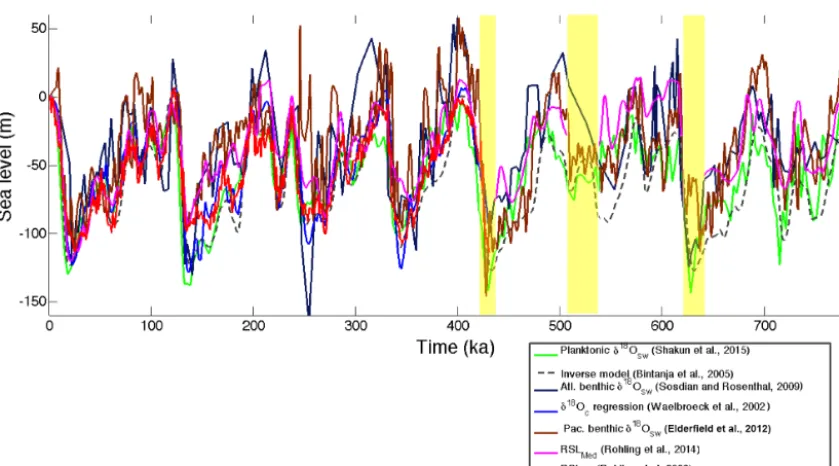
Figure 1.Eustatic and relative sea level estimates for the seven records on the LR04 age model (Lisiecki and Raymo, 2005). Yellow bars mark the sapropel layers removed from the Mediterranean RSL record (Rohling et al., 2014).
δ18Oc records is that the timing of benthicδ18Occhange at
different sites may differ by as much as 4 kyr during glacial terminations (Skinner and Shackleton, 2005; Lisiecki and Raymo, 2009; Stern and Lisiecki, 2014). The potential ef-fects of lags in benthic δ18Oc are evaluated using bootstrap
uncertainty analysis (Sect. 4.2).
For three reconstructions (Waelbroeck et al., 2002; Rohling et al., 2009, 2014) we aligned the individual sea level records with a preliminary sea level stack based on the other four sea level records on the LR04 age model. This was necessary because the local δ18Oc signals in semi-isolated
basins (Rohling et al., 2009, 2014) differ substantially from global mean benthic δ18Oc. In the coral-regression
recon-struction, Waelbroeck et al. (2002) pasted together portions of individual cores to form a preferred global composite. Al-though each core has benthicδ18Ocdata, generating new age
estimates for these cores could alter their δ18Oc regression
functions or create gaps or inconsistencies in the compos-ite. The procedure of aligning these three sea level records (Waelbroeck et al., 2002; Rohling et al., 2009, 2014) to a preliminary sea level stack should be approximately as accu-rate as the δ18Oc alignments. However, the direct sea level
alignments do have a slightly greater potential to align noise or local sea level variability.
After age models were adjusted, five of the records ended within the Holocene. Therefore, we appended a value of 0 m (i.e., present-day sea level) at 0 ka. In the two records which did end at 0 ka, modern sea level estimates were slightly be-low zero:−1.5 m (Bintanja et al., 2005) and−1.3 m (Rohling et al., 2014).
3.3 Principal component analysis
Principal component analysis (PCA) is commonly used to create stacks of paleoclimate data (e.g., Huybers and Wun-sch, 2004; Clark et al., 2012; Gibbons et al., 2014) and to quantify the common signal contained in core data. Synthe-sis is valuable because each record has its own assumptions and errors. If these records are all well-constrained measures of sea level, then PCA will reveal their respective levels of agreement or discrepancy. Additionally, PCA does not re-quire the assumption that each sea level record represents an independent measure of common signal. In contrast, a sea level estimate based on the unweighted mean of records would imply that uncertainties are uncorrelated across in-dividual reconstructions. While all records contain a strong ice volume signal, some of the non-ice volume signals are expected to correlate with one another. For example, as the
δ18O of ice sheet changes as it melts or freezes, the conver-sion from theδ18Osw to ice volume will be systematically
biased, whereas changes in the hydrological cycle may in-duce changes in the spatial variability ofδ18Oswat different
locations in the ocean.
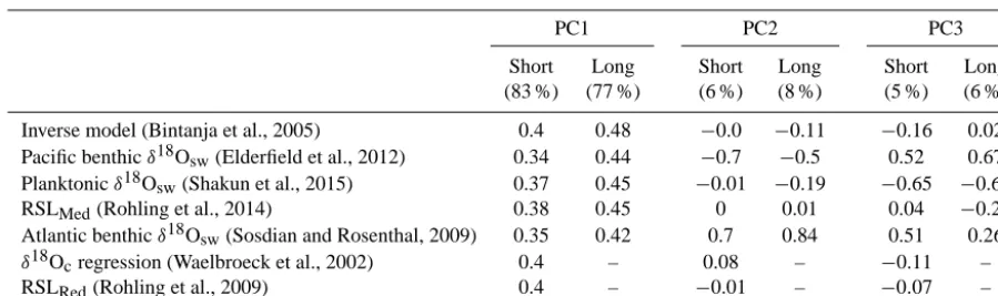
Table 1.Principal component analysis (PCA) loading for each proxy record. “Short” refers to the 0–430 ka time window, and “Long” refers to 0–798 ka. Numbers in parentheses give the percent variance explained by each principal component.
PC1 PC2 PC3
Short Long Short Long Short Long
(83 %) (77 %) (6 %) (8 %) (5 %) (6 %)
Inverse model (Bintanja et al., 2005) 0.4 0.48 −0.0 −0.11 −0.16 0.02 Pacific benthicδ18Osw(Elderfield et al., 2012) 0.34 0.44 −0.7 −0.5 0.52 0.67
Planktonicδ18Osw(Shakun et al., 2015) 0.37 0.45 −0.01 −0.19 −0.65 −0.65
RSLMed(Rohling et al., 2014) 0.38 0.45 0 0.01 0.04 −0.27
Atlantic benthicδ18Osw(Sosdian and Rosenthal, 2009) 0.35 0.42 0.7 0.84 0.51 0.26 δ18Ocregression (Waelbroeck et al., 2002) 0.4 – 0.08 – −0.11 –
RSLRed(Rohling et al., 2009) 0.4 – −0.01 – −0.07 –
and the threeδ18Oswrecords (Elderfield et al., 2012; Sosdian
and Rosenthal, 2009; Shakun et al., 2015) were scaled to eu-static sea level. However, for the planktonic stack we use the
δ18Osw record rather than the eustatic sea level conversion
because the sea level conversion involved detrending to make planktonicδ18Oc values agree with benthicδ18Oc. Because
PCA is designed to identify the common variance between the sea level proxies, it is preferable to keep the planktonic and benthicδ18Oswrecords independent of one another.
In the Mediterranean RSL record we removed putative sapropel layers at 434–452, 543–558, and 630–663 ka as vi-sually identified by Rohling et al. (2014). Because interpo-lating linearly across these gaps (Fig. 1) would bias sea level estimates towards higher lowstands for the glacial maxima occurring during these sapropel layers, we assumed that sea level remained constant at its pre-sapropel (glacial) level and then immediately jumped to the higher sea level values ob-served the ends of the sapropel layers (midway through the glacial terminations). Although this solution is not ideal, we must assume some sea level value at these times in order to include this record in the PCA.
Before PCA all seven records were interpolated to an even 1 ka time step. Then, to ensure equal weighting for each record in the PCA, each time series was normalized to a mean of zero and a standard deviation of one within each of the two time windows (0–430 and 0–798 ka). PCA was performed on seven records from 0 to 430 ka and five records from 0 to 798 ka (Fig. 2). Because PC1 produces similar loadings for each record (Table 1), the PC1 scores approximate the aver-age of all records for each point in time, which we refer to as a sea level stack.
We scaled the short and long stacks to eustatic sea level using an LGM value of −130 m at 24 ka based on a GIA-corrected coral compilation (Clark et al., 2009) and a Holocene value of 0 m at 5 ka. We scale the Holocene at 5 ka because eustatic sea level has been essentially constant for the past 5 ka (Clark et al., 2009), whereas the sea level stacks display a trend throughout the Holocene perhaps due to bio-turbation in the sediment cores. Scaling the sea level stack
based on the mid-Holocene (rather than 0 ka) should more accurately correct for the effects of bioturbation on previous interglacials because those highstand values have been sub-jected to mixing from both above and below. Finally, a com-posite sea level stack was created by joining the 0–430 ka stack with the 431–798 ka portion of the long stack after each was scaled to sea level. Because the two scaled sea level stacks produce similar values for 0–430 ka (Fig. 2), no cor-rection was needed to combine the records.
4 Uncertainty analysis
Because each of the records in the PCA is a sea level proxy and PC1 describes the majority of variance in the records, PC1 should represent the underlying common eustatic sea level signal in all proxies. PC1 describes 82 % of the variance in the seven records from 0 to 430 ka and 76 % of proxy vari-ance from 0 to 798 ka. Where the two time windows overlap (Fig. 2), the scaled sea level stacks have a root mean square error of only 3.4 m, thereby suggesting that the long stack is nearly as accurate as the short stack although it contains two fewer records. We assess the uncertainty of the scaled PC1 using multiple techniques: comparison with highstand and lowstand estimates from individual records (Sect. 4.1), com-parison with the unweighted mean of all records (Sect. 4.1), and use of bootstrapping and Monte Carlo-style random sam-pling (Sect. 4.2).
4.1 Mean sea level estimates
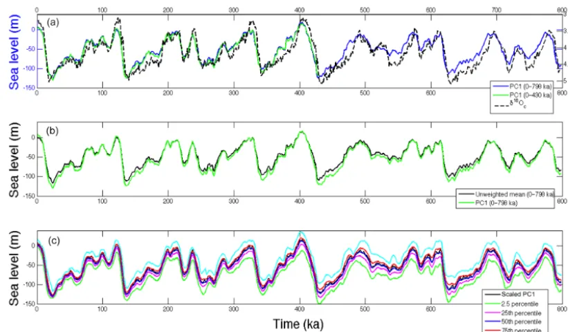
Figure 2.(a) Long and short sea level stacks compared to the LR04 benthicδ18Ocstack (Lisiecki and Raymo, 2005). (b) Scaled PC1
compared to unweighted mean of individual records. Scaled PC1 is comprised of short PC1 (0–431 ka) pasted to long PC1 (431–798 ka). (c) Scaled PC1 compared with percentile levels from the bootstrap results, which are also plotted as a composite of the short (0–431 ka) and long (431–798 ka) time windows.
were not used (e.g., extreme values at∼250 ka from ODP sites 1123 and 607).
Highstand sea level estimates vary widely between indi-vidual records with standard deviations of 11–26 m for each isotopic stage (Table 3). For example, individual estimates for MIS 11 at ∼400 ka vary between −5 and 57 m above modern, with a mean of 18 m and a standard deviation of 25 m. MIS 5e (119–126 ka) estimates range from−4 to 28 m above modern with a mean of 7 m and a standard deviation of 12 m. Generally, the highstand means have slightly greater amplitudes than our scaled stack; for example, the scaled stack estimates are 18 and 7 m for MIS 11 and MIS 5e, re-spectively. On the other hand, the mean of individual low-stands for the LGM (−123 m) underestimates eustatic sea level change, which is estimated to be −130 to −134 m (Clark et al., 2009; Lambeck et al., 2014).
The means of the individually picked highstands may be biased by the additive effects of noise. Conversely, the stack may underestimate sea level highstands if the individual age models are not properly aligned. The most definitive sea level estimates come from GIA-corrected coral compilations, which yield highstand estimates of 6–13 m above modern for MIS 11 (Raymo and Mitrovica, 2012) and 8–9.4 m for MIS 5e (Kopp et al., 2009). These values suggest that the stack may be more accurate for MIS 11 than MIS 5e, poten-tially because age model uncertainty would have less effect on the longer MIS 11 highstand. In contrast, MIS 5e may have consisted of two highstands each lasting only ∼2 ka
separated by several thousand years with sea level at or below modern (Kopp et al., 2013). Thus, the stack’s highstand esti-mates likely fail to capture short-term sea level fluctuations but rather reflect mean sea level during each interglacial.
To further test the sensitivity of our method, we compared the scaled PC1 with the unweighted mean of the seven in-terpolated sea level records (Fig. 2b). The unweighted-mean stack incorporates the same data as scaled PC1 except that it excludes Mediterranean estimates from sapropel intervals and uses the detrended sea level estimates from Shakun et al. (2015) instead of the rawδ18Osw data. The unweighted
stack closely resembles PC1 because the loadings of PC1 are very similar for all seven records (Table 1). However, the un-weighted stack underestimates LGM sea level, possibly be-cause some records (e.g., Rohling et al., 2009) may contain brief gaps at the glacial maximum. Thus, we prefer to scale PC1 to agree with well-constrained LGM sea level estimates. The scaled PC1 is in better agreement with the glacial sea level estimates of the unweighted five-record stack from 430 to 798 ka.
4.2 Bootstrapping and random sampling
Table 2.Sea level highstand and lowstand estimates from individual records (in meters above modern). See Table 1 for references. The last column gives the mean values from nine cores in Bates et al. (2014); these estimates were not included in our PCA.
Marine Age Inverse Pacific RSLRed RSLMed Planktonic Atlantic δ18Oc Bates et
Isotope (ka) model benthic δ18Osw benthic regression al. (2014)
Stage δ18Osw δ18Osw mean
2 18–25 −123 −113 −114 −120 −130 −124 −123 −133
5e 119–126 0 3 18 −4 −10 28 4.9 12
6 135–141 −123 −130 −99 −94 −138 −97 −129 −130
7a–c 197–214 −20 12 14 12 −16 34 −3.6 −3
7e 236–255 −18 16 −3 1 −20 −6.2 −9.4 −10
9 315–331 −0.5 40 11 −5 −27 43 5 8
10 342–353 −111 −96 −114 −77 −98 −112 −126 −122
11 399–408 0 58 4 12 −5 57 5.7 9
12 427–458 −126 −146 −118 – −142 −100 – −147
13 486–502 −29 18 – −8 −11 32 – −5
16 625–636 −126 −113 – – −144 −125 – −141
17 682–697 −23 31 – 0.5 −12 8.1 – −4
19 761–782 −21 21 – 7.2 1 −6.8 – −2
Table 3.Mean and standard deviation of sea level highstand and lowstand estimates (in meters above modern) from Table 2 compared to scaled PC1 and GIA-corrected estimates from corals and other coastal proxies. GIA-corrected estimates for MIS 2 are from Clark et al. (2009) and Lambeck et al. (2014), for MIS 5e from Dutton et al. (2015), and for MIS 11 from Raymo and Mitrovica (2012). Bootstrap 95 % confidence intervals are from sampling the seven-record-short PC1 for MIS 2–11 and from the five-record-long PC1 for MIS 12–19.
Marine Isotope Age range Standard Mean GIA- Scaled PC1 Scaled PC1 Bootstrap
Stage (ka) deviation corrected (0–430 ka) (0–798 ka) 95 % confidence interval
2 18–25 7 −123 −130 to−134 −130 −130 −136 to−128
5e 119–126 12 7 6 to 9 3 −1 −14 to 17
6 135–141 18 −118 – −123 −125 −142 to−111
7a–c 197–214 18 4 – −7 −5 −25 to 14
7e 236–255 11 −6 – −9 −13 −32 to−1
9 315–331 23 9 – −1 −2 −27 to 20
10 342–353 16 −107 – −108 −103 −128 to−92
11 399–408 25 18 6 to 13 16 19 −11 to 40
12 427–458 19 −130 – – −124 −163 to−100
13 486–502 22 −1 – – −11 −35 to 16
16 625–636 13 −130 – – −115 −149 to−87
17 682–697 19 0 – – −9 −28 to 15
19 761–782 14 0 – – −6 −25 to 10
δ18Oc alignments). We ran 1000 bootstrap iterations while
also performing random sampling to account for several of the uncertainties associated with our method. Before each it-eration of the bootstrapped PCA, we simulate the effects of uncertainty associated with our age model alignments by ap-plying an independent age shift of−2,−1, 0,+1, or+2 ka to each component record, with each potential value selected with equal probability. After performing each iteration of the PCA, we use random sampling to evaluate the effects of uncertainty associated with scaling PC1 to Holocene and LGM sea level. The particular Holocene point scaled to 0 m is randomly sampled from 0 to 6 ka with uniform distribu-tion. The LGM age is identified as the minimum sea level
in-terval for sea level maxima and minima in the bootstrapped samples.
5 The sea level contribution to benthicδ18Oc
The sea level stack and the LR04 benthic δ18Oc stack are
strongly correlated (r= −0.90). However, because δ18Oc
contains both an ice volume and temperature component, the
δ18Oc record has a greater amplitude than the ice
volume-drivenδ18Osw record. The spectral variance ofδ18Oswand δ18Ocin each orbital band can be used to determine the
rel-ative contributions of sea level and temperature variability in
δ18Oc. For this comparison, we convert the sea level stack to δ18Oswusing 0.009 ‰ m−1.
Although some studies have used 0.01 ‰ m−1(e.g., Sos-dian et al., 2009; Elderfield et al., 2012; Rohling et al., 2009), this conversion factor is likely too high for global mean
δ18Osw change at the LGM. Several lines of evidence
sug-gest an LGM δ18Osw change of 1–1.1 ‰ (Duplessy et
al., 2002; Adkins et al., 2002; Elderfield et al., 2012; Shakun et al., 2015), while LGM sea level was likely 125–134 m below modern (Clark et al., 2009; Lambeck et al., 2014; Rohling et al., 2014). These estimates suggest a conversion factor between 0.008 and 0.009 ‰ m−1. A conversion of 0.008 ‰ m−1would be consistent with aδ18Oice of−32 ‰
(Elderfield et al., 2012), similar to estimates for the Lauren-tide and Eurasian ice sheets (Duplessy et al., 2002; Bintanja et al., 2005; Elderfield et al., 2012). Therefore, 0.009 ‰ m−1 may be more appropriate when also considering changes in Greenland and Antarctic ice. However, the conversion factor between sea level and meanδ18Oswalso likely varies through
time as a result of changes in the mean isotopic content of each ice sheet (Bintanja et al., 2005) and their relative sizes.
Spectral analysis shows strong 100 and 41 ka peaks in both the LR04 benthicδ18Ocstack and the sea level stack (Fig. 3).
When converted toδ18Osw, the sea level stack contains 47 %
as much 100 ka power (0.009–0.013 ka−1 frequency band) as benthic δ18Oc and 37 % as much 41 ka power (0.024–
0.026 ka−1). The bootstrapped PC1 samples described in Sect. 4.2 are used to estimate 95 % confidence intervals (CIs) of 31–65 and 22–54 % for the relative power ofδ18Oswin the
100 and 41 ka bands, respectively. Considering all frequen-cies less than 0.1 ka−1,δ18Oswexplains 44 % (95 % CI=33–
57 %) of the variance inδ18Oc. Therefore, we estimate that
on average about 45 % of the glacial cycle variance in ben-thic δ18Oc derives from ice volume change and 55 % from
deep sea temperature change.
This∼45 % ice volume contribution to benthicδ18Oc is
smaller than the contribution estimated across the LGM to Holocene transition. An LGM sea level change of 130 m (Clark et al., 2009) should shift mean δ18Osw by 1.17 ‰,
whereas benthic δ18Oc changed by 1.79 ‰ (Lisiecki and
Raymo, 2005), suggesting that 65 % of the LGM δ18Oc
change was driven by ice volume. Many other studies have
Figure 3.Spectral analysis for composite sea level stack (scaled PC1) converted to itsδ18Oswcontribution using 0.009 ‰ m−1and
benthicδ18Ocstack (Lisiecki and Raymo, 2005) from 0 to 798 ka.
similarly found that the ice volume (δ18Osw) contribution
to δ18Oc is greatest during glacial maxima (Bintanja et
al., 2005; Elderfield et al., 2012; Rohling et al., 2014; Shakun et al., 2015). Additionally, theδ18Oswcontribution varies by
location, ranging from 0.7 to 1.37 ‰ based on glacial pore water reconstructions (Adkins et al., 2002). The wide vari-ability inδ18Oswbetween sites suggests that changes in deep
water formation processes (e.g., evaporation versus brine re-jection) greatly affect theδ18Oswsignal regionally or locally.
Therefore, theδ18Oswat a single site may differ considerably
from eustatic sea level.
6 Converting from benthicδ18Ocand sea level
Many studies have used benthicδ18Ocas a proxy for ice
vol-ume based on the argvol-ument that temperature and ice volvol-ume should be highly correlated through time (e.g., Imbrie and Imbrie, 1980; Abe-Ouchi et al., 2013). However, calculations based on the sea level stack spectral power and LGM-to-Holocene change suggest that ice volume change accounts for only 45–65 % of benthic δ18Oc glacial cyclicity
Addi-tionally, over the course of a glacial cycle the relative contri-butions of ice volume and temperature change dramatically, with temperature change preceding ice volume change (Bin-tanja et al., 2005; Elderfield et al., 2012; Shakun et al., 2015). Despite these complications the LR04 benthicδ18Ocstack is
strongly correlated with the sea level stack (r= −0.9). Here we explore more closely the functional relationship between benthic δ18Oc and sea level as inspired by Waelbroeck et
al. (2002).
Waelbroeck et al. (2002) solved for regression functions between several benthic δ18Oc records and coral elevation
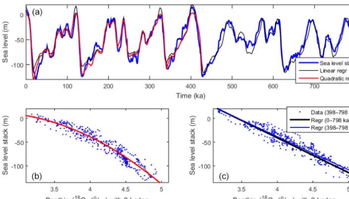
Figure 4.Comparison of benthicδ18Ocand sea level. (a) Linear and quadratic sea level models (Eqs. 1, 2, respectively) using smoothed
benthicδ18Oc(Lisiecki and Raymo, 2005) lagged by 2 ka. (b) Data from 0 to 397 ka with quadratic regression (red line). (c) Data from 398
to 798 ka with linear regression for 0–798 ka (black line) and 398–798 ka (blue line).
Figure 5.Second and third principal components for 0–430 and 0–798 ka. (a) Scores for PC2 largely reflect the difference between Atlantic and Pacific benthicδ18Osw. (b) Scores for PC3 largely reflect the difference benthic and planktonicδ18Osw. Dashed black line marks linear
trend from 0 to 430 ka.
LR04 global benthic stack with the sea level stack from 0 to 798 ka. One advantage of this comparison is that both records use the same age model. We evaluate whether a single re-gression can be used for the Late Pleistocene and identify a potential change in the relationship between benthic δ18Oc
and sea level at∼400 ka.
One difference between the two stacks is that the sea level stack is smoother (Fig. 2), likely because some of the sea level records are low resolution and all records were inter-polated to 1 ka spacing for PCA. Smoothing the LR04 stack using a 7 ka running mean improves the correlation between
benthicδ18Ocand sea level from−0.90 to−0.92.
Addition-ally, we estimate the phase lag between the two records by measuring their correlation with different time shifts. This analysis suggests a 2 ka phase lag between LR04 and the sea level stack, likely resulting from the fact that deep water tem-perature change leads ice volume change (e.g., Sosdian and Rosenthal, 2009; Elderfield et al., 2012; Shakun et al., 2015). When we apply this 2 ka lag to the smoothed LR04 stack, its correlation with sea level improves to−0.94.
level in meters (h) yields the equation
h= −73x+251 (1)
(Fig. 4, black line). Using the bootstrapped PC1 samples described in Sect. 4.2 and Monte Carlo-style sampling of smoothing windows that range from 0 to 7 kyr and lags from 0 to 3 kyr, we find that the 95 % CI for the slope of this re-gression is −56 to −79 m ‰−1. The root mean square er-ror (RMSE) for this model is 10.7 m (95 % CI =9–22 m), but the fit is better for the older portion of the record (398– 798 ka, RMSE=10.2 m) than the more recent portion (0– 397 ka, RMSE=11.2 m). In particular, the linear model esti-mates sea levels that are 10–20 m too high during most high-stands and lowhigh-stands back to MIS 10 at∼345 ka. The dif-ference in fit before and after 398 ka is somewhat dependent upon the assumed lag between benthicδ18O and sea level; the linear model fits the older portion of the record better in 84 % of samples with a 3 ka lag but only 61 % of sampled regressions with no lag. The effect of a smaller lag is mainly to increase the RMSE of the older portion of the linear re-gression from a mean of 12.7 m (3 ka lag) to 15.7 m (no lag). A plot of sea level versus the smoothed and lagged benthic
δ18Oc (Fig. 4b) suggests that the relationship between the
two is approximately quadratic
h= −26x2+135x−163 (2)
from 0 to 397 ka (RMSE=9.4 m, 95 % CI=8–22 m) and linear from 398 to 798 ka. This transition appears to take place between 360 and 400 ka because MIS 11 clearly falls on the linear trend whereas MIS 10 is a much better fit by the quadratic equation (Fig. 4a). Because this transition occurs after MIS 11, the extreme duration or warmth of this inter-glacial might have played an important role in the transition. A change in the relationship between benthicδ18Oc and
sea level could be caused by a change in the mean isotopic content of ice sheets or the relationship between ice volume and deep water temperature (possibly also global surface temperature). Interglacials after MIS 11 were likely warmer or had more depleted δ18Osw relative to ice volume.
Simi-larly, glacial maxima were probably warmer and/or had less
δ18Osw change. Combined changes in temperature and
iso-topic fractionation may be the most likely explanation since warmer ice sheets also probably have less depletedδ18Oice.
In fact Antarctic ice cores are isotopically less depleted dur-ing MIS 5e and MIS 9 than MIS 11 (Jouzel et al., 2007). Additionally, Antarctic surface temperatures and CO2levels
were similar for all three interglacials (Masson-Delmotte et al., 2010; Petit et al., 1999) despite the smaller ice volume during MIS 11.
There is little direct evidence to explain the changing rela-tionship betweenδ18Ocand sea level during glacial maxima
because glacial values for both deep water temperature and the isotopic composition of Antarctic ice are similar through-out the last 800 ka (Elderfield et al., 2012; Masson-Delmotte
et al., 2010). The change in glacial maxima after 400 ka could be caused by less depletedδ18Oice in Northern Hemisphere
(NH) ice sheets. Although no long records of NHδ18Oice
ex-ist, global mean SST was 0.5–1◦C warmer during MIS 2, 6, and 8 than during MIS 12 (Shakun et al., 2015). Alterna-tively, the apparent linear trend between sea level andδ18Oc
during glacial maxima before 400 ka (Fig. 4c) could be an artifact of poor sea level estimates for MIS 12 and 16, which may be biased 10–20 m too high (Table 3) by missing data during sapropel intervals in the Mediterranean RSL record (Rohling et al., 2014).
In conclusion, a systematic relationship can be defined between Late Pleistocene benthic δ18Oc and sea level, and
the functional form of this relationship likely changed af-ter MIS 11. Change in theδ18Oc–sea-level relationship
dur-ing interglacials likely results from warmer high latitudes with less depletedδ18Oice after 400 ka. Glacial maxima
af-ter 400 ka may also have been warmer with less depleted NHδ18Oice, but this apparent change during glacial
max-ima could be an artifact of bias in the sea level stack during MIS 12 and 16. Changes in the relationship between benthic
δ18Ocand sea level are also likely to have occurred during
the early or mid-Pleistocene. For example, the same regres-sion probably would not apply to the 41 ka glacial cycles of the early Pleistocene (Tian et al., 2003).
7 Differences between sea level proxies
Whereas PC1 tells us about the common variance between the sea level proxies, PC2 and PC3 tell us about their dif-ferences. PC2 represents 6 and 8 % of the variance for the short and long time windows, respectively. The scores and loads are similar for both analyses (Fig. 5, Table 1) except for a sign change; therefore, we multiply by−1 the scores and loads of PC2 and PC3 of the short time window. Large PC2 loadings with opposite sign contributions for the 1123 and 607 benthicδ18Oswrecords suggest that PC2 represents
differences in theδ18Oswof deep water in the Atlantic and
Pacific basins. Most notably, PC2 has a strong peak at ap-proximately 250 ka (Fig. 5), associated with very low values in the 607 benthicδ18Oswrecord and very high values in the
1123 benthicδ18Oswrecord (Fig. 1).
PC3 captures 5 % of the variance in the 430 ka stack and 6 % of the variance in the 798 ka stack. Unlike PC1 and PC2, the loads vary between the short and long PC3 (Table 1); here we focus on the short version because it contains more proxy records. In the 430 ka stack, PC3 is most highly represented by the planktonicδ18Oswstack with a load of−0.7 and the
1123 and 607 benthicδ18Oswrecords with loads of about 0.5.
These loads suggest that PC3 dominantly reflects planktonic versus benthic differences inδ18Osw. PC3 scores exhibit a
linear trend from 0 to 430 ka, which supports the findings of previous studies that suggest planktonic δ18Osw should
Shakun et al., 2015). Furthermore, PC3 suggests that ben-thic δ18Osw may also need to be detrended in the opposite
direction. This effect could be caused by long-term changes in the hydrologic cycle or deep water formation processes, which lead to a change in the partitioning of oxygen isotopes between the surface and deep ocean.
8 Conclusions
PCA indicates a strong common sea level signal in the seven records analyzed for 0–430 ka and five records for 0–798 ka. Furthermore, the similarity between the short and long stacks indicates that the longer stack with five records is nearly as good an approximation of sea level as the seven-record stack. Sea level estimates for each interglacial vary greatly between records, producing standard deviations of 11–26 m. Gener-ally, the mean for each individual highstand is greater in mag-nitude than our stack estimate. Based on comparison with GIA-corrected coral sea level estimates for MIS 5e and 11, the stack likely reflects mean sea level for each interglacial and fails to capture brief sea level highstands, such as those lasting only∼2 ka during MIS 5e (Kopp et al., 2013).
A comparison of individual records shows that highstand and lowstand estimates have a mean standard deviation of 17 m (for MIS 5e–19). Uncertainty in the stack is estimated using bootstrapping and random sampling, which yields a mean standard deviation for scaled PC1 of 9.4 m with seven records (0–430 ka) and 12 m with five records (0–798 ka). The bootstrap uncertainty estimates also include age uncer-tainty; however, this systematically smooths the bootstrap re-sults and, thus, underestimates individual highstands relative to both individual records and scaled PC1 (Fig. 2c).
We estimate that sea level change accounts for only about 45 % of the orbital-band variance in benthicδ18Oc, compared
to 65 % of the LGM-to-Holocene benthic δ18Oc change.
Nonetheless, benthic δ18Oc is strongly correlated with sea
level (r= −0.9). If LR04 benthic δ18Oc stack is smoothed
and lagged by 2 ka, the relationship between benthicδ18Oc
and sea level is well-described by a linear function from 398 to 798 ka and a quadratic function from 0 to 398 ka. In partic-ular, interglacials MIS 9 and 5e, which had larger ice sheets than MIS 11, appear to have been as warm (or warmer) as MIS 11 with isotopically less depleted ice sheets.
The second and third principal components of the sea level records describe differences between the proxies. PC2 repre-sents the difference between theδ18Oswof deep water in the
Atlantic and Pacific basins; a peak in PC2 scores at 250 ka indicates large differences between the basins at this time. PC3 represents the differences between planktonic and ben-thicδ18Oswrecords and suggests a linear trend between the
two from 0 to 430 ka. Thus,δ18Oswrecords vary across ocean
basins and between the surface and the deep. In conclusion, the stack of sea level proxies presented here should be a more
accurate eustatic sea level record than any of the individual records it contains.
Data availability
The sea level stack is archived in the Supplement and at the World Data Center for Paleoclimatology operated by the Na-tional Climatic Data Center of the NaNa-tional Oceanographic and Atmospheric Association (https://www.ncdc.noaa.gov/ paleo/study/19982).
The Supplement related to this article is available online at doi:10.5194/cp-12-1079-2016-supplement.
Acknowledgements. We thank all researchers who made their data available. Additionally, we thank David Lea, Jeremy Shakun, Alex Simms, Charles Jones, and Leila Carvalho for beneficial discussions.
Edited by: E. Wolff
References
Abe-Ouchi, A., Saito, F., Kawamura, K., Raymo, M. E., Okuno, J., Takahashi, K., and Blatter, H.: Insolation-driven 100,000-year glacial cycles and hysteresis of ice-sheet volume, Nature, 500, 190–193, doi:10.1038/nature12374, 2013.
Adkins, J. F., McIntyre, K., and Schrag, D. P.: The Salinity, Temper-ature, andδ18O of the Glacial Deep Ocean, Science, 298, 1769– 1773, doi:10.1126/science.1076252, 2002.
Andersen, M. B., Stirling, C. H., Potter, E. K., Halliday, A. N., Blake, S. G., Mc-Culloch, M. T., Ayling, B. F., and O’Leary, M.: High-precision U-series measurements of more than 500,000 year old fossil corals, Earth Planet. Sc. Lett., 265, 229–245, 2008. Bard, E., Hamelin, B., Fairbanks, R. G., and Zindler, A.: Calibration of the14C timescale over the past 30,000 years using mass spec-trometric U–Th ages from Barbados corals, Nature, 345, 405-410, 1990.
Bard, E., Hamelin, B., Arnold, M., Montaggioni, L., Cabioch, G., Faure, G., and Rougerie, F.: Deglacial sea-level record from Tahiti corals and the timing of global meltwater discharge, Na-ture, 382, 241–244, doi:10.1038/382241a0, 1996.
Bates, S. L., Siddall, M., and Waelbroeck, C.: Hydrographic variations in deep ocean temperature over the mid-Pleistocene transition, Quaternary Sci. Rev., 88, 147–158, doi:10.1016/j.quascirev.2014.01.020, 2014.
Bintanja, R., Roderik, S. W., and van de Wal, O. J.: Modeled atmo-spheric temperatures and global sea levels over the past million years, Nature, 437, 125–128, doi:10.1038/nature03975, 2005. Blanchon, P., Eisenhauer, A., Fietzke, J., and Liebetrau, V.:
Boak, E. H. and Turner, I. L.: Shoreline Definition and Detection: A Review, J. Coastal Res., 214, 688–703, doi:10.2112/03-0071.1, 2005.
Bowen, D. Q.: Sea level ∼400 000 years ago (MIS 11): ana-logue for present and future sea-level?, Clim. Past, 6, 19–29, doi:10.5194/cp-6-19-2010, 2010.
Bryden, H. L. and Kinder, T. H.: Steady two-layer exchange through the Strait of Gibraltar, Deep-Sea Res., 38, Supplement 1, S445– S463, 1991.
Clark, P. U., Dyke, A. S., Shakun, J. D., Carlson, A. E., Clark, J., Wohlfarth, B., Mitrovica, J. X., Hostetler, S. W., and Mc-Cabe, A. M.: The Last Glacial Maximum, Science, 325, 710– 714, doi:10.1126/science.1172873, 2009.
Clark, P. U., Shakun, J. D., Baker, P. A., Bartlein, P. J., Brewer, S., Brook, E., Carlson, A. E., Cheng, H., Kaufman, D. S., Liu, Z., Marchitto, T. M., Mix, A. C., Morrill, C., Otto-Bliesner, B. L., Pahnke, K., Russell, J. M., Whitlock, C., Adkins, J. F., Blois, J. L., Clark, J., Colman, S. M., Curry, W. B., Flower, B. P., He, F., Johnson, T. C., Lynch-Stieglitz, J., Markgraf, V., McManus, J., Mitrovica, J. X., Moreno, P. I., and Williams, J. W.: Global climate evolution during the last deglaciation, P. Natl. Acad. Sci. USA, 109, E1134–E1142, doi:10.1073/pnas.1116619109, 2012. Creveling, J. R., Mitrovica, J. X., Hay, C. C., Austermann, J., and Kopp, R. E.: Revisiting tectonic corrections applied to Pleis-tocene sea-level highstands, Quaternary Sci. Rev., 111, 72–80, doi:10.1016/j.quascirev.2015.01.003, 2015.
Duplessy, J. C., Labeyrie, L., and Waelbroeck, C.: Constraints on the ocean isotopic enrichment between the Last Glacial Maxi-mum and the Holocene: Paleoceanographic implications, Qua-ternary Sci. Rev., 21, 315–330, 2002.
Dutton, A. and Lambeck, K.: Ice Volume and Sea Level During the Last Interglacial, Science, 337, 216–220, 2012.
Dutton, A., Carlson, A., Long, A., Milne, G., Clark, P., DeConto, R., Horton, B. P., Rahmstorf, S., and Raymo, M.: Sea-level rise due to polar ice-sheet mass loss during past warm periods, Science, 349, 6244, aaa4019–1, doi:10.1126/science.aaa4019, 2015. Dwyer, G. S., Cronin, T. M., Baker, P. A., Raymo, M. E.,
Buzas, J. S., and Corrige, T.: North Atlantic Deepwa-ter Temperature Change During Late Pliocene and Late Quaternary Climatic Cycles, Science, 270, 1347–1351, doi:10.1126/science.270.5240.1347, 1995.
Edwards, R. L., Beck, J. W., Burr, G. S., Donahue, D. J., Chappell, J. M. A., Bloom, A. L., Druffel, E. R. M., and Taylor, F. W.: A Large Drop in Atmospheric14C/12C and Reduced Melting in the Younger Dryas, Documented with230Th Ages of Corals, Sci-ence, 260, 962–968, 1993.
Elderfield, H., Ferretti, P., Greaves, M., Crowhurst, S. J., Mc-Cave, I. N., Hodell, D. A., and Piotrowski, A. M.: Evo-lution of ocean temperature and ice volume through the Mid-Pleistocene Climate Transition, Science, 337, 704–709, doi:10.1126/science.1221294, 2012.
Fairbanks, R. G.: A 17,000 year glacio-eustatic sea level record: influence of glacial melting rates on the Younger Dryas event and deep-ocean circulation, Nature, 342, 637–642, 1989. Ganopolski, A. and Calov, R.: The role of orbital forcing, carbon
dioxide and regolith in 100 kyr glacial cycles, Clim. Past, 7, 1415–1425, doi:10.5194/cp-7-1415-2011, 2011.
Gibbons, F. T., Oppo, D. W., Mohtadi, M., Rosenthal, Y., Cheng, J., Liu, Z., and Linsley, B. K.: Deglacialδ18O and hydrologic
variability in the tropical Pacific and Indian Oceans, Earth Planet. Sci. Lett., 387, 240–251, 2014.
Govin, A., Braconnot, P., Capron, E., Cortijo, E., Duplessy, J.-C., Jansen, E., Labeyrie, L., Landais, A., Marti, O., Michel, E., Mos-quet, E., Risebrobakken, B., Swingedouw, D., and Waelbroeck, C.: Persistent influence of ice sheet melting on high northern lat-itude climate during the early Last Interglacial, Clim. Past, 8, 483–507, doi:10.5194/cp-8-483-2012, 2012.
Grant, K. M., Rohling, E. J., Bronk Ramsey, C., Cheng, H., Edwards, R. L., Florindo, F., Heslop, D., Marra, F., Roberts, A. P., Tamisiea, M. E., and Williams, F.: Sea-level variabil-ity over five glacial cycles, Nature Communications, 5, 5076, doi:10.1038/ncomms6076, 2014.
Hanebuth, T., Stattegger, K., and Grootes, P. M.: Rapid Flooding of the Sunda Shelf: A Late-Glacial Sea-Level Record, Science, 288, 1033–1035, doi:10.1126/science.288.5468.1033, 2000. Hay, C., Mitrovica, J. X., Gomez, N., Creveling, J. R., Austermann,
J., and Kopp, R. E.: The sea-level fingerprints of ice-sheet col-lapse during interglacial periods, Quaternary Sci. Rev., 87, 60– 69, doi:10.1016/j.quascirev.2013.12.022, 2014.
Horton, B. P.: Late Quaternary Relative Sea-level Changes in Mid-latitudes, in: Encyclopedia of Quaternary Science, edited by: Elias, S. A., Elsevier, Boston, MA, 2064–3071, 2006.
Huybers, P. and Wunsch, C.: A depth-derived Pleistocene age model: Uncertainty estimates, sedimentation variability, and nonlinear climate change, Paleoceanography, 19, 1–24, doi:10.1029/2002PA000857, 2004.
Imbrie, J. and Imbrie, J. Z.: Modeling the climatic response to or-bital variations, Science, 207, 943–953, 1980.
Jouzel, J., Masson-Delmotte, V., Cattani, O., Dreyfus, G., Falourd, S., Hoffmann, G., Minster, B., Nouet, J., Barnola, J. M., Chap-pellaz, J., Fischer, H., Gallet, J. C., Johnsen, S., Leuenberger, M., Loulergue, L., Luethi, D., Oerter, H., Parrenin, F., Raisbeck, G., Raynaud, D., Schilt, A., Schwander, A., Selmo, E., Souchez, R., Spahni, R., Stauffer, B., Steffensen, J. P., Stenni, B., Stocker, T. F., Tison, J. L., Werner, M., and Wolff, E. W.: Orbital and Mil-lennial Antarctic Climate Variability over the Past 800,000 Years, Science 317, 793–796, doi:10.1126/science.1141038, 2007. Kopp, R. E., Simons, F. J., Mitrovica, J. X., Maloof, A. C.,
and Oppenheimer M.: Probabilistic assessment of sea level during the last interglacial stage, Nature, 462, 863–867, doi:10.1038/nature08686, 2009.
Kopp, R. E., Simons, F. J., Mitrovica, J. X., Maloof, A. C., and Op-penheimer, M.: A probabilistic assessment of sea level variations within the last interglacial stage, Geophys. J. Int., 193, 711–716, 2013.
Lambeck, K., Rouby, H., Purcell, A., Sun, Y., and Sambridge, M.: Sea level and global ice volumes from the Last Glacial Maximum to the Holocene, P. Natl. Acad. Sci. USA, 111, 15296–15303, doi:10.1073/pnas.1411762111, 2014.
Lea, D. W., Martin, P. A., Pak, D. K., and Spero, H. J.: Reconstruct-ing a 350 ky history of sea level usReconstruct-ing planktonic Mg/Ca and oxygen isotope records from a Cocos Ridge core, Quaternary Sci. Rev., 21, 283–293, doi:10.1016/S0277-3791(01)00081-6, 2002. Lisiecki, L. E. and Lisiecki, P. A.: Application of dynamic
Lisiecki, L. E. and Raymo, M. E.: A Pliocene-Pleistocene stack of 57 globally distributed benthicδ18O records, Paleoceanography, 20, PA1003, doi:10.1029/2004PA001071, 2005.
Lisiecki, L. E. and Raymo, M. E.: Diachronous benthicδ18O re-sponses during late Pleistocene terminations, Paleoceanography, 24, PA3210, doi:10.1029/2009PA001732, 2009.
Martin, P. A., Lea, D. W., Rosenthal, Y., Shackleton, N. J., Sarnthein, M., and Papenfuss, T.: Quaternary deep sea tem-perature histories derived from benthic foraminiferal Mg/Ca, Earth Planet. Sc. Lett., 198, 193–209, doi:10.1016/S0012-821X(02)00472-7, 2002.
Masson-Delmotte, V., Stenni, B., Jouzel, J., Landais, A., Röthlis-berger, R., Minster, B., Hansen, J., Pol, K., Barnola, J. M., Miko-lajewicz, U., Braconnot, P., Chappellaz, J., Otto-Bliesner, B., Cattani, O., and Krinner, G.: EPICA Dome C record of glacial and interglacial intensities, Quaternary Sci. Rev., 29, 113–128, 2010.
Medina-Elizalde, M.: A global compilation of coral sea-level benchmarks: Implications and new challenges, Earth Planet. Sc. Lett., 362, 310–318, doi:10.1016/j.epsl.2012.12.001, 2013. Muhs, D. R., Meco, J., Simmons, K. R.: Uranium-series ages
of corals, sea level history, and palaeozoogeography, Ca-nary Islands, Spain: An exploratory study for two Quater-nary interglacial periods, Palaeogeogr. Palaeocl., 394, 99–118, doi:10.1016/j.palaeo.2013.11.015, 2014.
National Climatic Data Center: https://www.ncdc.noaa.gov/paleo/ study/19982, last access: 20 April 2016.
Petit, J. R., Jouzel, J., Raynaud, D., Barkov, N. I., Barnola, J.-M., Basile, I., Bender, M., Chappellaz, J., Davisk, M., Delaygue, G., Delmotte, M., Kotlyakov, V. M., Legrand, M., Lipenkov, V. Y., Lorius, C., Pépin, L., Ritz, C., Saltzman, E., and Stievenard, M.: Climate and atmospheric history of the past 420,000 years from the Vostok ice core, Antarctica, Nature, 399, 429–436, 1999. Raymo, M. E. and Mitrovica, J. X.: Collapse of polar ice
sheets during the stage 11 interglacial, Nature, 483, 453–456, doi:10.1038/nature10891, 2012.
Raymo M. E., Ruddiman W. F., Shackleton N. J., and Oppo D. W.: Evolution of Atlantic Pacificδ13C Gradients over the Last 2.5 My, Earth Planet. Sc. Lett., 97, 353–368, 1990.
Rohling, E. J., Grant, K., Bolshaw, M., Roberts, A. P., Siddall, M., Hemleben, C., and Kucera, M.: Antarctic temperature and global sea level closely coupled over the past five glacial cycles, Nat. Geosci., 2, 500–504, 2009.
Rohling, E. J., Grant, K. M., Bolshaw, M., Roberts, A. P., Sid-dall, M., Hemleben, C., Kucera, M., Foster, G. L., Marino, G., Roberts, A. P., Tamisiea, M. E., and Williams, F.: Sea-level and deep-sea-temperature variability over the past 5.3 million years, Nature, 508, 477–482, 2014.
Schiebel, R., Zeltner, A., Treppke, U. F., Waniek, J. J., Bollmann, J., Rixen, T., and Hemleben, C.: Distribution of diatoms, coccolithophores and planktic foraminifera in the Arabian Sea, Mar. Micropaleontol., 51, 345–371, doi:10.1016/j.marmicro.2004.02.001, 2004.
Shackleton, N. J.: Attainment of isotopic equilibrium between ocean water and the benthonic foraminifera genus Uvigerina: Isotopic changes in the ocean during the last glacial, in: Collo-ques internationaux, Centre national de la recherche scientifique, France, 219, 203–209, 1974.
Shakun, J. D., Lea, D. W., Lisiecki, L. E., and Raymo, M. E.: An 800-kyr record of global surface oceanδ18O and implications for ice volume-temperature coupling, Earth. Planet. Sc. Lett., 426, 58–68, 2015.
Siddall, M., Smeed, D. A., Hemleben, Ch., Rohling, E. J., Schmeltzer, I., and Peltier, W. R.: Understanding the Red Sea re-sponse to sea level, Earth. Planet. Sc. Lett., 225, 421–434, 2004. Siddall, M., Hönisch, B., Waelbroeck, C., and Huybers, P.: Changes in deep Pacific temperature during the mid-Pleistocene transition and Quaternary, Quaternary Sci. Rev., 29, 170–181, 2010. Skinner, L. C. and Shackleton, N. J.: An Atlantic lead over Pacific
deep-water change across Termination I: implications for the ap-plication of the marine isotope stage stratigraphy, Quaternary Sci. Rev., 24, 571–580, doi:10.1016/j.quascirev.2004.11.008, 2005.
Sosdian, S. and Rosenthal, Y.: Deep-Sea Temperature and Ice Vol-ume Changes Across the Pliocene-Pleistocene Climate Tran-sitions, Science, 325, 306–310, doi:10.1126/science.1169938, 2009.
Stein, M., Wasserburg, G. J., Aharon, P., Chen, J. H., Zhu, Z. R., Bloom, A., and Chappell, J.: TIMS U-series dating and stable isotopes of the last interglacial event in Papua New Guinea, Geochimica et Cosmochimica Acta, 57, 11, 2541–2554, doi:10.1016/0016-7037(93)90416-T, 1993.
Stern, J. V. and Lisiecki, L. E.: Termination 1 timing in radiocarbon dated regional benthicδ18O stacks, Paleoceanography, 29, 1127– 1142, doi:10.1002/2014PA002700, 2014.
Stirling, C. H., Esat, T. M., McCulloch, M. T., and Lambeck, K.: High-precision U-series dating of corals from Western Australia and implications for the timing and duration of the Last Inter-glacial, Earth Planet. Sc. Lett., 135, 115–130 doi:10.1016/0012-821X(95)00152-3, 1995.
Thompson, W. G. and Goldstein, S. L.: Open-System Coral Ages Reveal Persistent Suborbital Sea-Level Cycles, Science, 308, 401–404, doi:10.1126/science.1104035, 2005.
Tian, L., Yao, T., Schuster, P. F., White, J. W. C., Ichiyanagi, K., Pendall, E., Pu, J., and Yu, W.: Oxygen-18 concentrations in re-cent precipitation and ice cores on the Tibetan Plateau, J. Geo-phys. Res., 108, 4293, doi:10.1029/2002JD002173, 2003. Waelbroeck, C., Labeyrie, L., Michel, E., Duplessy J.C., McManus
J.: Sea-level and deep water temperature changes derived from benthic foraminifera isotopic records, Quaternary Sci. Rev., 21, 295–305, 2002.