Extended Two-Phase Algorithm for Fast Discovery of High Utility Itemsets on Probabilistic Databases and Possible Application of Counting Inference Approach

(1)

Extended Two-Phase Algorithm for Fast Discovery of High Utility Itemsets on

Probabilistic Databases and Possible Application of Counting Inference

Approach

Niket BhargavaA, Dr. Manoj ShuklaB

Ȧ

Department of Computer Science and Engineering, Mewar University, Chittaurgarh, India

Ḃ

Department of Electronics and Communication Engineering, Rajiv Gandhi Technical University, Bhopal, India

Abstract

Traditional association rules mining cannot meet the demands arising from some real applications. Such domains are like the mining of sensor data, geographical system data, biological data. These domain suffer from uncertain data. To capture inherent uncertainty probabilistic databases were introduced. In contrast to the traditional data mining algorithm, by considering the different values of individual items as utilities, utility mining focuses on identifying the itemsets with high utilities. In this paper, we presented n extension to Two-Phase algorithm that is extended to mine probabilistic high utility patterns, to efficiently prune down the number of candidates and precisely obtain the complete set of high utility itemsets, transaction weighted utility, high utility, counting inference, and probability threshold are used. It performs very efficiently in terms of speed and memory cost both on synthetic and real databases, even on large databases that are difficult for existing algorithms to handle when the algorithm is run using counting inference when it is applicable.

Keywords: High Utility Mining, Probabilistic Databases, Counting Inference, Key Patterns, Non-Key Patterns.

I. INTRODUCTION

Traditional Association rules mining (ARM) [1] model treat all the items in the database equally by only considering if an item is present in a transaction or not. Frequent itemsets identified by ARM may only contribute a small portion of the overall profit, whereas non-frequent itemsets may contribute a large portion of the profit. In reality, a retail business may be interested in identifying its most valuable customers (customers who contribute a major fraction of the profits to the company). These are the customers, who may buy full priced items, high margin items, or gourmet items, which may be absent from a large number of transactions because most customers do not buy these items. In a traditional frequency oriented ARM, these transactions representing highly profitable customers may be left out. Utility mining is likely to be useful in a wide range of practical applications[10]. In this paper we discuss two mode separately and try to put real world utilization of concepts possible. In first, we use the systems which can be valued using their presence or absence, can be easily extended to opt the counting inference model under anti-monotonicity defined. Second, when the items are present in non-binary quantity in each case. For this second case, we will use general Apriori like level wise approach.

Modern field of business application of technology like data mining, big data, data science are evolved to give insights and to predict in future and to suggest prescriptions to improve profit. In mining we use measure utility to evaluate usefulness. A utility mining model was defined in [2]. Utility is a measure of how much “useful” an itemset is. The goal of utility mining is to identify high utility itemsets that drive a large portion of the total utility. Traditional ARM problem is a special case of utility

mining, where the utility of each item is always 1 and the sales quantity is either 0 or 1 [10]. we will extend this model and use non binary sales quantity and show that counting inference can be utilized.

There is no efficient strategy to find all the high utility itemsets due to the non-existence of “downward closure property” (anti-monotone property) in the utility mining model. A heuristics [2] is used to predict whether an itemset should be added to the candidate set. This algorithm has been named as MEU (Mining using Expected Utility) for the paper which is one among the motivation for the work presented here[10]. However, the prediction usually overestimates, especially at the beginning stages, where the number of candidates approaches the number of all the combinations of items. Such requirements can easily overwhelm the available memory space and computation power of most of the machines. In addition, MEU may miss some high utility itements when the variance of the itemset supports is large. The challenge of utility mining is in restricting the size of the candidate set and simplifying the computation for calculating the utility. In order to tackle this challenge, concept of transaction weighted utility was introduced in [10]. This is known as Two-Phase algorithm to efficiently mine high utility itemsets.

(2)

II. RELATED WORK A. Utility Mining Two Phase Algorithm

Researches that assign different weights to items have been proposed in [60, 61, 62, 63]. These weighted ARM models are special cases of utility mining. A concept, itemset share, is proposed in [64]. It can be regarded as a utility because it reflects the impact of the sales quantities of items on the cost or profit of an itemset. Several heuristics have been proposed. A utility mining algorithm is proposed in [65], where the concept of “useful” is defined as an itemset that supports a specific objective that people want to achieve. The definition of utility and the goal of his algorithm are different from those in our work.

1) Two-Phase Algorithm

We start with the definition of a set of terms that leads to the formal definition of utility mining problem. The same terms are given in [2]. Let say, I = {i1, i2, …, im} is a set of items and D = {T1, T2, …, Tn} be a transaction database where each transaction Ti  D is a subset of I. Than,

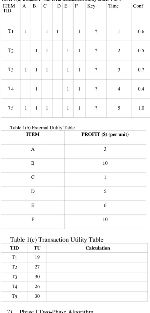
 o(ip, Tq), local transaction utility value, represents the quantity of item ip in transaction Tq. For example, o(A, T5) = 1, in Table 1(a). Note, that here we are taking all local transaction utility as 1. These values can be any integer value, represents the count of item in transaction respectively [67].

 s(ip), external utility, is the value associated with item ip in the Utility Table. This value reflects the importance of an item, which is independent of transactions. For example, in Table 1(b), the external utility of item F, s(F), is 10.

 u(ip, Tq), utility, the quantitative measure of utility for item ip in transaction Tq, is defined as o(ip,Tq) 

s(ip). For example, u(A, T5) = 1  3 = 1, in Table 1  u(X, Tq), utility of an itemset X in transaction Tq, is

defined as u(ip,Tq) , where summation is over all ipX

X = {i1, i2, …, ik} is a k-itemset, X Tq and 1km.

 u(X), utility of an itemset X, is defined as



u( X

,Tq) . (1.1)

Tq



D



X



_Tq

Utility mining is to find all the itemsets whose utility values are beyond a user specified threshold. An itemset X is a high utility itemset if u(X X I and low utility itemset. For example, in Table 1, u({A, E}) = u({A, E}, T3) + u({A, E}, T5) = {3,6} 9+ {3,6} 9 = 18. drawbacks in MEU, Two-Phase algorithm was proposed [67]. This algorithm works in two phases. In Phase I, was defined transaction-weighted utilization measure and proposed a model ─ transaction-weighted utilization mining. This model maintains a Transaction-weighted Downward Closure Property. Thus, only the

combinations of high transaction-weighted utilization itemsets are added into the candidate set at each level during the level-wise search. Phase I may overestimate some low utility itemsets, but it never underestimates any itemsets. In phase II, only one extra database scan is performed to filter the overestimated itemsets [67]. Table 1(a) Database with local transaction utility either 1 or 0

ITEM TID

A B C D E F Key Time Conf

T1 1 1 1 1 ? 1 0.6

T2 1 1 1 1 ? 2 0.5

T3 1 1 1 1 1 ? 3 0.7

T4 1 1 1 ? 4 0.4

T5 1 1 1 1 1 ? 5 1.0

Table 1(b) External Utility Table

ITEM PROFIT ($) (per unit)

A 3

B 10

C 1

D 5

E 6

F 10

Table 1(c) Transaction Utility Table

TID TU Calculation

T1 19

T2 27

T3 30

T4 26

T5 30

2) Phase I Two-Phase Algorithm

These definitions were introduced in Two-Phase algorithm [67]

Definition 1. (Transaction Utility) The transaction utility of transaction Tq, denoted as tu(Tq), is the sum of the utilities of all the items in Tq: tu(Tq ) 

(3)

(c) gives the transaction utility for each transaction in Table 1.

Definition 2. (Transaction-weighted Utilization) The transaction-weighted utilization of an itemset X, denoted as twu(X), is the sum of the transaction utilities of all the transactions containing X:

twu( X ) 



tu(Tq) 

 X Tq Dq

For the example in Table 1, twu(AD) = tu(T3) + tu(T5) = 30 + 30 = 60, and for pattern AC in Table1 twu(AC) =t u(T1) + tu(T3) + tu(T5) = 19 + 30 + 30 = 79

Definition 3. (High Transaction-weighted Utilization Itemset) For a given itemset X, X is a high transaction-weighted utilization itemset if twu(X)  ’, where ’ is the user specified threshold.

Theorem 1. (Transaction-weighted Downward Closure Property) Let Ik be a k- itemset and Ik-1 be a (k -1)-itemset such that Ik-1  Ik. If Ik is a high transaction- weighted utilization itemset, Ik-1 is a high transaction-weighted utilization itemset.

The Transaction-weighted Downward Closure

Property indicates that any superset of a low transaction-weighted utilization itemset is low in transaction-transaction-weighted utilization. That is, only the combinations of high transaction-weighted utilization (k-1)- itemsets could be added into the candidate set Ck at each level.

Theorem 2. Let HTWU be the collection of all high transaction-weighted utilization itemsets in a transaction database D, and HU be the collection of high utility itemsets in D. If ’= , then HU HTWU.

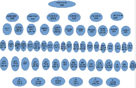
According to Theorem 2, we can utilize the Transaction-weighted Downward Closure Property in our transaction-weighted utilization mining in Phase I by assuming ’ =  and prune those overestimated itemsets in Phase II. Figure 1 shows the search space of Phase I. The level-wise search stops at the third level, one level less than MEU. (For larger databases, the savings should be more evident.) Transaction-weighted utilization mining model outperforms MEU in several aspects:

1)Less candidates ─ When ’ is large, the search space can be significantly reduced at the second level and higher levels. As shown in Figure 1, four out of 10 itemsets are pruned because they all contain item A. However, in MEU, the prediction hardly prunes any itemset at the beginning stages.

2)Accuracy ─ Based on Theorem 2, if we let ’=, the complete set of high utility itemsets is a subset of the high transaction-weighted utilization itemsets discovered by our transaction-weighted utilization mining model. However, MEU may miss some high utility itemsets when the variation of itemset supports is large.

3)Arithmetic complexity ─ One of the kernel operations

in the Two-Phase algorithm is the calculation for each item set's transaction-weighted utilization as in

equation 1.2, which only incurs add operations rather than a number of multiplications in MEU. Thus, the overall computation is much less complex.

3) Phase II of Two-Phase Algorithm

In Phase II, one database scan is performed to filter the high utility itemsets from high transaction-weighted utilization itemsets identified in Phase I. The number of high transaction-weighted utilization itemsets is small when twu is high. Hence, the time saved in Phase I may compensate for the cost incurred by the extra scan in Phase II.

B. Probabilistic Association Rule Mining

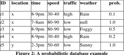
In this section we will discuss mining uncertain database data with probabilistic certainty. Data uncertainty is inherent in many applications such as sensor monitoring systems, location-based services, and biological databases. To manage this vast amount of imprecise information, probabilistic databases have been recently developed. In this paper, we study the discovery of frequent patterns and association rules from probabilistic data under the Possible World Semantics. This is technically challenging, since a probabilistic database can have an exponential number of possible worlds. The data managed in many emerging applications is often uncertain. Integration and record linkage tools, for example, associate confidence values to the output tuples according to the quality of matching [34]. In structured information extractors, confidence values are appended to rules for extracting patterns from unstructured data [52]. In habitat monitoring systems, data collected from sensors like temperature and humidity are noisy [34]. The locations of users obtained through RFID and GPS systems are also imprecise [25, 39]. To handle these problems, probabilistic databases have been recently proposed, where uncertainty is treated as a “first-class citizen” [31, 34, 44, 33, 38]. Due to its simplicity in database design and query semantics, the tuple-uncertainty model is commonly used in probabilistic databases. Conceptually, each tuple carries an existential probability attribute, which denotes the confidence that the tuple exists. Figure 2 illustrates this model, which records traffic violation events due to red-light running. The details of each event (e.g., location, and traffic volume) are captured

(4)

by a red-light camera system, which contains sensors and cameras mounted in road intersections. Each tuple is annotated by a probability that a true violation happens. The probability that a violation occurs is determined by sensor measurement errors, as well as the uncertainty caused by automatic information extraction of the photographs taken by the system [53].

ID location time speed traffic weather prob.

t1 x 8-9pm 30-40 high Rain 0.1 t2 x 7-8am 80-90 low null 1.0 t3 x 8-9pm 80-90 low Foggy 0.5 t4 x 8-9pm 30-40 high Rain 0.2 t5 y 2-3pm 50-60 low Sunny 1.0

Figure 2: A probabilistic database example

To interpret tuple uncertainty, the Possible World Semantics (or PWS in short) is often used [34]. Conceptually, a database is viewed as a set of deterministic instances (called possible worlds), each of which contains a set of zero or more tuples. A possible world for Figure 2 consists of the tuples { t2, t3, t5 }, existing with a probability of (1 - 0.1) x 1.0 x 0.5 x ( 1 - 0.2) x 1.0 = 0.036. Any query evaluation algorithm for probabilistic database has to be correct under PWS. That is, the results produced by the algorithm should be the same as if the query is evaluated on every possible world[34] Although PWS is intuitive and useful, evaluating queries under this notion is costly. This is because a probabilistic database has an exponential number of possible worlds. For example, the table in Figure 1 has 23 = 8 possible worlds. Performing query evaluation or data mining under PWS can thus be technically challenging. In fact, the mining of uncertain or probabilistic data has recently attracted research attention [26]. In [41], efficient clustering algorithms were developed to group uncertain objects that are close to each other. Recently, a Naive Bayes classifier has been developed [49]. The goals of this paper are: (1) propose a definition of frequent patterns and association rules for the tuple uncertainty model; and (2) develop efficient algorithm for mining frequent patterns and association rules.

Association rule Probability

r1: {location=x} ⇒ {time=8-9pm}

r2: {location=x} ⇒ {speed=80-90,traffic=low}

0.15 0.49

Figure 3: Sample p-ARs derived from Figure 2

The frequent patterns discovered from probabilistic data are also probabilistic, to reflect the confidence placed on the mining results. Figure 3 shows two probabilistic frequent patterns (or p-FP) extracted from the database in Figure 2. A p-FP is a set of attribute values that occur frequently with sufficiently high probabilities. The pmf of the number of tuples is the support count that contains a pattern with specific probability. Under PWS, a database is

a set of possible worlds, each of which records a (different) support of the same pattern. Hence, the support of a frequent pattern is a pmf. In figure 1, if we consider all possible worlds where { location = x }occurs three times, the pmf of { location = x } with a support of 3 is 0.49. for the p-FP shown. Figure 3 displays their related probabilistic association rules (or p-ARs). Here, rule r2 suggests that with a 0.49 probability, 1) red-light violations occur frequently at location x and 2) when this happens, the involved vehicle is likely driving at a high speed amid low traffic. We will later explain more about the semantics of p-FP and p-AR. A simple way of finding p-FPs is to extract frequent patterns from every possible world. This is practically infeasible, since the number of possible worlds is exponentially large.

Prior work. [30] studied approximate frequent

patterns on noisy data, while [42] examined association rules on fuzzy sets. The notion of a “vague association rule” was developed in [43]. These solutions were not developed on probabilistic data models. For probabilistic databases, [32, 25] derived patterns based on their expected support counts. [54, 50] found that the use of expected support may render important patterns missing. They discussed the computation of the probability that a pattern is frequent. While [55] handled the mining of single items, our solution can discover patterns with more than one item. The data model used in [50] assumes that for each tuple, each attribute value has a probability of being correct. This is different from the tuple-uncertainty model, which describes the joint probability of attribute values within a tuple. pmf evaluation method DC algorithm is asymptotically faster than the DP algorithms used in [54, 50], and is thus more scalable for large and dense datasets. To our best knowledge, none of the above works considered the important problem of generating association rules on probabilistic databases.

This section is organized as follows. Section 3.1 introduces the notions of p-FPs and p-ARs. Sections 3.2 present our algorithms for mining p-FPs. Section 3.3 discusses fully solved example using dataset used in paper introduced Pascal algorithm. The CIPFP algorithm is described in section 5 and example is described in section 6

C. Problem Definition

We first review frequent patterns and association rules in Sections 3.1.1. Then, we discuss the uncertain data model in Section 3.1.2. We present the problems of mining p-FPs and p-ARs, in Sections 3.1.3 and 3.1.4.

(5)

sup(X) minsup (1)

where minsup ∈ N ∩ [1, n] is the support threshold [27].

Given patterns X and Y (with X∩Y = Ø), if pattern XY is frequent, then X is also frequent (called the anti-monotonicity property). Also, X⇒Y is an association rule if following conditions holds:

supp(XY) ≥ minsup (2)

supp(XY)/supp(X) ≥ minconf (3)

sup(XY) / sup(X), denoted by conf(X⇒Y), is the confidence of X⇒Y, and minconf ∈ R ∩ (0, 1] is the confidence threshold. To verify Equation 3, the values of sup(XY) and sup(X) have to be found first. We remark that a transaction database is essentially a relational table with asymmetric binary attribute values. For example, the existence of item “apple” in a transaction is equivalent to a binary attribute of a tuple with a value of 1. This kind of attributes, assumed in this paper, is also considered by some mining algorithms (e.g., [27, 28]). To handle other attribute types (e.g., continuous and categorical), discretization and binarization techniques can be used to convert them to binary attributes [52].

2) The Possible World Semantics

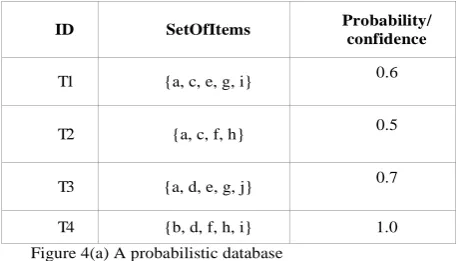
We assume that each transaction has an existential probability, which specifies the chance that the transaction exists. Figure 4(a) illustrates this database, in which each transaction is a set of items represented by letters. This model has been used to capture uncertainty in many applications, including data streams[33] and geographical services[45].

Now, let P(E) be the probability that an event E occurs and PDB be probabilistic database of size n. Also, let Ti (where i = 1, ..., n ) be the ID of each tuple in PDB. Suppose Ti.S is the set of items contained in Ti, and Ti.p is the existential probability of Ti.

ID SetOfItems Probability/ _confidence

T 1 {a, c, e, g, i} 0.6

T 2 {a, c, f, h} 0.5

T 3 {a, d, e, g, j} 0.7

T 4 {b, d, f, h, i} 1.0

Figure 4(a) A probabilistic database

Under PWS, PDB is a set of possible worlds W. Figure 4(b) lists all possible worlds for figure 4(a). Each Wi ε W exists with probability P(Wi). For

example P(W2) = T1.p X ( 1 – T2.p) X ( 1 -T3.p) X T4.p or 0.09. The sum of possible world probabilities is one. Also, the number of possible worlds is exponentially large, i.e. |w| = O( 2n). Our goal is to discover patterns and rule using these possible worlds.

W Tuples in W Prob. W Tuples in W Prob.

W1 T4 0.06 W5 T1, T2, T4 0.09

W2 T1, T4 0.09 W6 T1, T3, T4 0.21

W3 T2, T4 0.06 W7 T2, T3, T4 0.14

W4 T3, T4 0.14 W8 T1, T2, T3, T4 0.21 Figure 4(b) Possible World for PDB in Figure 4(a)

3) Probabilistic Frequent Patterns

we first explain the concept of support for probabilistic data. Given a pattern X, we denote its support in each world Wi as supi(X) is obtained by counting the number of times X appears in Wi. Since each Wi exists with a probability, the support of X in PDB, i.e. sup(X), is a random variable. We denote fX(k) that the probability mass function (pmf) of sup(X) can take. Specifically, fX(k) is the probability that sup(X) = k, and fX(k) = 0 for any k ∉ [0,n]. We use an array to store the non-zero values of fX, where fX[k] = P(supp(X) = k). Figure 4(c) depicts the support pmf of {a}. the probability that sup({a}) = 1 is 0.29.

DEFINITION 1. A pattern X is a probabilistic frequent pattern or p-FP in PDB if

P(sup(X) ≥ minsup) ≥ minprob (4)

where minprob є R ∩ (0,1] is the probability threshold.

Problem 1 (p-FP Mining). Given PDB, minsup and minprob, return a set of {X, fX(k), where X is a FP .As we will discuss, the pmfs obtained with p-FPs are essential to generating probabilistic association rules. There are methods to approximating and compressing pmfs (e.g., see [35]). Here we assume that the pmf is exact, but our solutions can be extended to support these schemes. Next, we present a useful lemma.

(6)

Lemma 1 (Anti-monotonicity). If pattern X is a p-FP, then any pattern X' ⊂ X is also a p-FP.

The anti-monotonicity property is true for frequent patterns in exact data [27]. Lemma 1 allows us to stop examining a pattern, if any of its sub-pattern is not a p-FP. A p-FP X is said to be maximal if we cannot find another p-FP Y such that X ⊂ Y . A maximal p-FP can succinctly represent a set of p-FPs when their supports are not concerned. Since the mining of maximal frequent patterns is an important problem [28] for exact data, we also study maximal p-FPs, together with free set, maximal set make a complete system, we study them too,:

Problem 2.1 (Free set p-FP Mining). Given a database PDB, minsup and minprob, return all minimal generators or free sets p-Fps.

Problem 2.2 (Maximal p-FP Mining). Given a database PDB, minsup and minprob, return all maximal p-Fps.

Problem 2.3 (closed p-FP Mining). Given a database PDB, minsup and minprob, return all closed p-FPs.

4) Probabilistic Association Rules

In a probabilistic database, the support counts of patterns are random variables. Let P (X⇒Y) be the probability that X⇒Y is an association rule. By Equations 2 and 3, we have:

P (X⇒Y) = P [sup(XY ) > minsup∧ conf (X⇒Y) ≥ minconf] (5)

Definition 2. X⇒Y is a probabilistic association rule (p-AR in short) if

P (X ⇒ Y ) ≥ minprob (6)

The problem of p-AR mining is defined as follows.

Problem 3 (p-AR Mining). Given minsup, minprob, minconf, and the p-FPs and their support pmfs obtained from Problem 1, derive all p-ARs and their probabilities.

A simple way of solving Problems 1, 2, and 3 is to expand PDB into all possible worlds, compute patterns and rules from each world, and then combine the results. If minsup=2, minconf=0.5, and minprob=0.2, for Figure 4(a), {a}⇒{c} is an association rule only in worlds W5 and W8 (Figure 4(c)), with P ({a}⇒{c}= Pr(W5) + Pr(W 8) = 0.09 + 0.21 = 0.3. Since this is larger than 0.2, {a}⇒{c} is a p-AR. This method is not practical , due to the large number of possible worlds. To tackle Problems 1 and

2, proposed algorithms, namely probabilistic Apriori discussed and solved fully in next section 4.

5) Counting Inference Approach

Counting inference approach is a Pattern counting inference mechanism that minimize as much as possible the number of pattern support counts performed when extracting frequent patterns. It is based on the notion of key patterns, where a key pattern is minimal pattern of equivalence class gathering all patterns common to the same objects of the database relation. With pattern counting inference, only the supports of the frequent key patterns (and some infrequent ones) are determined from the database, while supports of the frequent non key pattern are derived from those of the frequent key patterns. Definitions for Key patterns and pattern Counting Inference are as following;

Definition 1.3.1. Let P be a finite set of items, O a finite set of objects (e.g., transaction ids) and RO  P a binary relation (where (o, p)  R may be read as “item p is included in transaction o”).The triple D=(O, P, R) is called dataset [12]. Each subset p of P is called a pattern. We say that a Pattern P is included in an object o  O if (o,p)  R for all p  P[].Let f be the function which assign to each pattern pP the set of all objects which include this pattern :f(P) = { o  O| o includes P }. The support of a pattern P is given by supp (P) = card (f (P))/card (O). For a given threshold minsup [0,1], a pattern P is called frequent pattern if supp(P)≥ minsup.

Definition 1.3.2. A K- pattern p is a subset of P with card (P) = K .A candidate K-pattern where all its proper sub-patterns are frequent. [12]

Definition 1.3.3. For patterns P, Q  P let PθQ if and only if f (P) =f (Q) .the set of patterns which are equivalent to a pattern P is given by [P] = {Q  P | Pθ Q}[12]

Definition 4 A pattern P is a key pattern if P  min [P]. A candidate key pattern is a pattern where all its proper sub patterns are frequent key patterns.

Theorem 3.2.1 (i ) if Q is a key pattern and P  Q ,then P is also a key pattern.(ii) if P is not a key pattern and, P  Q then Q is not a key pattern either.[12]

Theorem 3.2.2. Let P be a pattern.(i) Let p P .then P  [P \{p}] if and only if supp(P)= supp(P\ {p}), (ii) P is a key pattern if and only if supp(P) ≠ min p P (supp(P\{p})) [12]

Theorem 3.2.3 Let P is a non key pattern then supp(P)= min p P (supp(P\{p}))[12]

II. OUR ALGORITHM : CIPU

Five steps for CIPU – Probabilistic High Utility Itemset Mining are as follows:

a. Phase I of Two Phase twu pruning

(7)

c. Phase 3 minprob pruning over actual high utility patterns, As we have for given observe support we have twu and utility, for high utility at given support the probability of existence of transaction can be filtered out, to give most probabilistic high utility itemsets list.

d. if Presence/Absence data item entry for step “a.” CIPFP, TempCIPFP can be used, with a modification for twu to act as support for Key-Pattern, Non-Key Pattern evaluation. e. for others use a, b, and c step.

III. RUNNING EXAMPLE The database to be operated upon is as following; TABLE 3.1

TID A B C D E F Key Time Conf Transaction

utility tu(Tq)

T1 1 1 1 1 ? 1 0.6 19

T2 1 1 1 1 ? 2 0.5 27

T3 1 1 1 1 1 ? 3 0.7 30

T4 1 1 1 ? 4 0.4 26

T5 1 1 1 1 1 ? 5 1.0 30

Step 3a Phase I will be as following; a.1 calculate traction utility for all transactions in database see last column in table 3.1.

TABLE 3.2 UTILITY TABLE

A B C D E F

3 10 1 5 6 10

a.2 for 1-itemsset in I, calculate transaction weighted utility as follows; mintwu = minutil= 20.

TABLE 3.3 1-item set TID,Item belongs to

Sum tu of TIDs twu of 1-itemset Remark calculate tu using DB scan The tu 1-items et twu >= mint wu Use to make candi date in next step

{A} T1, T3, T5 19+30+30 79 > mintwu 9 ? No {B} T2, T3, T4, T5 27+30+26

+30

113 > mintwu 40 ? Yes

{C} T1, T2, T3, T5 19+27+30 +30

106 > mintwu 4 ? No

{D} T1 19 19 < mintwu 6 ? No {E} T2, T3, T4, T5 27+30+26

+30

{F} T1, T2, T3, T4, T5

19+27+30 +26+30

a.2 for 2-itemsset calculate transaction weighted utility as follows; mintwu = minutil= 20.

TABLE 3.4 2-itemse t TID, Item belong s to Sum tu of TIDs twu of 1-item set Remark calculate tu using DB scan

The tu 1-itemset twu >=mintw u Use to make candi date in next step

{AB} T3,T5 30+30 26 > mintwu 26 ? Yes {AC} T1,T3,

T5

19+30+ 30

12 > mintwu 12 ? No

{AD} T1 19 19 < mintwu 8 ? No {AE} T3,T5 30+30 60 > mintwu 18 ? No {AF} T1,T3,

T5

19+30+ 30

{BC} T2,T3, T5

27+30+ 30

{BD} - - - -

{BE} T2,T3, T4,T5

27+30+ 26+30

{BF} T2,T3, T4,T5

27+30+ 26+30

{CD} T1 19 19 < mintwu 6 ? No {CE} T2,T3,

T5

27+30+ 30

{CF} T1,T2, T3,T5

19+27+ 30+30

{DE} - - - -

{DF} T1 19 19 < mintwu 15 ? No {EF} T2,T3,

T4,T5 27+30+ 26+30

TABLE 3.4 3-itemset TID, Item belongs to Sum tu of TIDs twu of 1-itemse t Remar k calcula te tu using DB scan The tu 1-itemset twu >=mintw u Use to make candi date in next step

{ABC} T3,T5 30+30 60 > mintwu

28 ? Yes

{ABD} - - - -

{ABE} T3,T5 30+30 60 > mintwu

36 ? Yes

{ABF} T3,T5 30+30 60 > mintwu

35 ? Yes

{ACD} T1 19 19 < mintwu

9 ? No

{ACE} T3,T5 30+30 60 > mintwu

20 ? Yes

{ACF} T1,T3,T5 30+30 60 > mintwu

42 ? Yes

(8)

{ADF} T1 19 19 < mintwu

18 ? No

{AEF} T3,T5 30+30 60 > mintwu

36 ? Yes

{BCD} - - - -

{BCE} T2,T3,T5 27+30 +30

87 > mintwu

51 ? Yes

{BCF} T2,T3,T5 27+30 +30

87 > mintwu

63 ? Yes

{BDE} - - - -

{BDF} - - - -

{BEF} T2,T3,T4 ,T5

27+30 +26+3 0

113 > mintwu

104 ? Yes

{CDE} - - - -

{CDF} T1 19 19 < mintwu

16 ? No

{CEF} T2,T3,T5 30+30 60 > mintwu

51 ? Yes

{DEF} - - - -

TABLE 3.5 4-itemset TID

Item belong s to Su m tu of TID s twu of 1-itemse t Remark calculate tu using DB scan The tu 1-itemset twu >=mintw u Use to make candida te in next step

{ABCD} - - - -

{ABCE} T3,T5 30+ 30

{ABCF} T3,T5 30+ 30

{ABDE} - - - -

{ABDF} - - - -

{ABEF} T3,T5 30+ 30

{ACDE} - - - -

{ACDF} T1 19 19 < mintwu 19 ? No {ACEF} T3,T5 30+

30

{ADEF} - - - -

{BCDE} - - - -

{BCDF} - - - -

{BCEF} T2,T3, T5

27+ 30+ 30

{BDEF} - - - -

{CDEF} - - - -

TABLE 3.6 5-itemset TID

Item belong s to Sum tu of TIDs twu of 1-item set Remark calculate tu using DB scan The tu 1-itemset twu >= mintwu Use to make candidate in next step

{ABCDE} - - - -

{ABCDF} - - - -

{ABCEF} T3,T5 30+30 60 > mintwu 60 ? Yes

{ABDEF} - - - -

{ACDEF} - - - -

{BCDEF}

- - - -

TABLE 3.7

1-itemset TID

, Ite m belo ngs to Sum tu of TID s twu of 1-items et Remark calculate tu using DB scan The tu 1-itemset twu >= mintwu

Use to make candidate in next step

{ABCDEF} - - - -

A total of 62 candadate set of items are possible if level by level chronologically orders itemsets are considered. Depending upon itemset for k = 1 to 6, for each k-itemset 6+15+20+14+6+1 = 62. Depending upon twu mintwu thresold the search space consist of only 5+10+10+4+1+0 = 30 patterns need to be scanned against database instead of 62. when performed database scan to calculate exact utility for the 30 frequent twu items, the high utility itemsets found are 3+8+8+5+1+0 = 25. for these 25 patters for their highest count support probability in PWS we can compare against minprob. And can find probabilistic utility itemset as final answer.

IV. CONCLUSION

(9)

REFERENCES

[1] R. Agrawal, C. Faloutsos, and A. Swami. Efcient similarity search in sequence databases. In Proc. of the Fourth International Conference on Foundations of Data Organization and Algorithms, Chicago, October 1993.

[2] R. Agrawal, S. Ghosh, T. Imielinski, B. Iyer, and A. Swami. An interval classi er for database mining applications. In Proc. of the VLDB Conference, pages 560{573, Vancouver, British Columbia, Canada, 1992.

[3] R. Agrawal, T. Imielinski, and A. Swami. Database mining: A performance perspective. IEEE Transactions on Knowledge and Data En- gineering, 5(6):914{925, December 1993. Special Issue on Learning and Discovery in Knowledge- Based Databases. [4] R. Agrawal, T. Imielinski, and A. Swami. Mining association rules

between sets of items in large databases. In Proc. of the ACM SIGMOD Con- ference on Management of Data, Washington, D.C., May 1993.

[5] R. Agrawal and R. Srikant. Fast algorithms for mining association rules in large databases. Re- search Report RJ 9839, IBM Almaden Research Center, San Jose, California, June 1994.

[6] D. S. Associates. The new direct marketing. Business One Irwin, Illinois, 1990.

[7] R. Brachman et al. Integrated support for data archeology. In AAAI-93 Workshop on Knowledge Discovery in Databases, July 1993.

[8] L. Breiman, J. H. Friedman, R. A. Olshen, and C. J. Stone. Classi cation and Regression Trees. Wadsworth, Belmont, 1984. [9] P. Cheeseman et al. Autoclass: A bayesian classi cation system. In

5th Int'l Conf. on Machine Learning. Morgan Kaufman, June 1988. [10] D. H. Fisher. Knowledge acquisition via incremental conceptual

clustering. Machine Learning, 2(2), 1987.

[11] J. Han, Y. Cai, and N. Cercone. Knowledge discovery in databases: An attribute oriented approach. In Proc. of the VLDB Conference, pages 547{559, Vancouver, British Columbia, Canada, 1992. [12] M. Holsheimer and A. Siebes. Data mining: The search for

knowledge in databases. Technical Report CS-R9406, CWI, Netherlands, 1994.

[13] M. Houtsma and A. Swami. Set-oriented mining of association rules. Research Report RJ 9567, IBM Almaden Research Center, San Jose, Cali- fornia, October 1993.

[14] R. Krishnamurthy and T. Imielinski. Practi- tioner problems in need of database research: Re- search directions in knowledge discovery. SIG- MOD RECORD, 20(3):76{78, September 1991.

[15] P. Langley, H. Simon, G. Bradshaw, andJ. Zytkow. Scienti c Discovery: Computational Explorations of the Creative Process. MIT Press, 1987.

[16] H. Mannila and K.-J. Raiha. Dependency inference. In Proc. of the VLDB Conference, pages 155{158, Brighton, England, 1987. [17] H. Mannila, H. Toivonen, and A. I. Verkamo. E cient algorithms

for discovering association rules. In KDD-94: AAAI Workshop on Knowl- edge Discovery in Databases, July 1994.

[18] S. Muggleton and C. Feng. E cient induction of logic programs. In S. Muggleton, editor, Inductive Logic Programming. Academic Press, 1992.

[19] J. Pearl. Probabilistic reasoning in intelligent systems: Networks of plausible inference, 1992.

[20] G. Piatestsky-Shapiro. Discovery, analysis, and presentation of strong rules. In G. Piatestsky-Shapiro, editor, Knowledge Dis- covery in Databases. AAAI/MIT Press, 1991. [21] G. Piatestsky-Shapiro, editor. Knowledge Dis- covery in

Databases. AAAI/MIT Press, 1991.

[22] J. R. Quinlan. C4.5: Programs for Machine Learning. Morgan Kaufman, 1993.

[23] Rakesh Agrawal, Ramakrishnan Srikant: “Fast Algorithms for Mining Association Rules” Proceedings of the 20th VLDB Conference Santiago, Chile, 1994

[24] Liwen Sun, Reynold Cheng, David W. Cheung, Jiefeng Cheng, “Mining Uncertain Data with Probabilistic Guarantees”, KDD’10, July 25–28, 2010, Washington, DC, USA. Copyright 2010 ACM 978-1-4503-0055-1/10/07

[25] A. Deshpande et al. Model-driven data acquisition in sensor networks. In VLDB, 2004.

[26] C. Aggarwal, Y. Li, J. Wang, and J. Wang. Frequent pattern mining with uncertain data. In KDD, 2009.

[27] C. Aggarwal and P. Yu. A survey of uncertain data algorithms and applications. IEEE Transactions on Knowledge and Data Engineering, 21(5), 2009.

[28] R. Agrawal and R. Srikant. Fast algorithms for mining association rules in large databases. Technical report, RJ 9839, IBM, 1994. [29] R. Bayardo, Jr. Efficiently mining long patterns from databases. In

SIGMOD, 1998.

[30] D. Burdick, M. Calimlim, J. Flannick, J. Gehrke, and T. Yiu. MAFIA: A maximal frequent itemset algorithm. IEEE Transactions on Knowledge and Data Engineering, 17, 2005. [31] H. Cheng, P. Yu, and J. Han. Approximate frequent itemset mining

in the presence of random noise. Soft Computing for Knowledge Discovery and Data Mining, 2008.

[32] R. Cheng, D. Kalashnikov, and S. Prabhakar. Evaluating probabilistic queries over imprecise data. In SIGMOD, 2003. [33] C. K. Chui, B. Kao, and E. Hung. Mining frequent itemsets from

uncertain data. In PAKDD, 2007.

[34] G. Cormode and M. Garofalakis. Sketching probabilistic data streams. In SIGMOD, 2007.

[35] N. Dalvi and D. Suciu. Efficient query evaluation on probabilistic databases. In VLDB, 2004.

[36] M. Garofalakis and A. Kumar. Wavelet synopses for general error metrics. ACM Transactions on Database Systems, 30(4), 2005. [37] K. Gouda and M. J. Zaki. GenMax: An efficient algorithm for

mining maximal frequent itemsets. Data Mining and Knowledge Discovery, 11(3), 2005.

[38] R. Hogg, A. Craig, and J. Mckean. Introduction to Mathematical Statistics (6th ed.). Prentice Hall, 2004.

[39] J. Huang et al. MayBMS: A Probabilistic Database Management System. In SIGMOD, 2009.

[40] N. Khoussainova, M. Balazinska, and D. Suciu.Towards correcting input data errors probabilistically using integrity constraints. In MobiDE, 2006.

[41] D. Knuth. The art of computer programming, vol. 3.Addison Wesley, 1998.

[42] H. Kriegel and M. Pfeifle. Density-based clustering of uncertain data. In KDD, 2005.

[43] C. Kuok, A. Fu, and M. Wong. Mining fuzzy association rules in databases. SIGMOD Record, 1998.

[44] A. Lu, Y. Ke, J. Cheng, and W. Ng. Mining vague association rules. In DASFAA, 2007.

[45] M. Mutsuzaki et al. Trio-one: Layering uncertainty and lineage on a conventional dbms. In CIDR, 2007.

[46] M. Yiu et al. Efficient evaluation of probabilistic advanced spatial queries on existentially uncertain data. IEEE Transactions on Knowledge and Data Engineering, 21(9), 2009.

[47] R. Motwani and P. Raghavan. Randomized algorithms. Cambridge University Press, New York, NY, USA, 1995.

[48] A. Oppenheim, R. Schafer, and J. Buck. Discrete-time signal processing (2nd ed.). Prentice Hall, 1999.

[49] P. Sistla et al. Querying the uncertain position of moving objects. In Temporal Databases: Research and Practice. Springer Verlag, 1998.

[50] J. Ren, S. Lee, X. Chen, B. Kao, R. Cheng, and D. Cheung. Na¨ıve Bayes Classification of Uncertain Data. In ICDM, 2009.

[51] T. Bernecker et al. Probabilistic frequent itemset mining in uncertain databases. In KDD, 2009.

[52] T. Jayram et al. Avatar information extraction system. IEEE Data Engineering Bulletin, 29(1), 2006.

[53] P. Tan, M. Steinbach, and V. Kumar. Introduction to Data Mining. Pearson Education, 2006.

(10)

[55] Q. Zhang, F. Li, and K. Yi. Finding frequent items in probabilistic data. In SIGMOD, 2008.

[56] M.H.Dunham. Data Mining: Introductory and Advanced Topics. Prentice Hall, 2003.

[57] Y Li, P Ning, XS Wang, S Jajodia “ Discovering calendar- based temporal association rule “Data & Knowledge Engineering, 2003 - Elsevier

[58] Bastide, R Taouil, N Pasquier, G Stumme, “Levelwise Search of Frequent Patterns with Counting Inference “ACM SIGKDD Explorations Newsletter, 2000

[59] Hong Yao, Howard J. Hamilton, and Cory J. Butz: A Foundational Approach to Mining Itemset Utilities from Databases. SDM (2004) [60] C.H. Cai, Ada W.C. Fu, C.H. Cheng, and W.W. Kwong: Mining

Association Rules with Weighted Items. IDEAS (1998)

[61] W. Wang, J. Yang, and P. Yu: Efficient Mining of Weighted Association Rules (WAR). 6th KDD (2000)

[62] Feng Tao, Fionn Murtagh, and Mohsen Farid: Weighted Association Rule Mining using Weighted Support and Significance Framework. 9th KDD (2003)

[63] S. Lu, H. Hu, and F. Li: Mining weighted association rules. Intelligent Data Analysis, 5(3) (2001), 211-225

[64] B. Barber and H.J.Hamilton: Extracting share frequent itemsets with infrequent subsets. Data Mining and Knowledge Discovery, 7(2) (2003), 153-185

[65] Raymond Chan, Qiang Yang, Yi-Dong Shen: Mining high utility Itemsets. ICDM (2003)

[66] IBM data generator,

http://www.almaden.ibm.com/software/quest/Resources/index.shtm l