New Wavelet Transform Denoising Algorithm
Anumula.Janardhan
Professor ECE Department, JITSWarangal-AP , India
Prof.K.Kishan Rao
Director, V C E Warangal-AP , IndiaAbstract-- Denoising based on Wavelet Transform (WT) is simple and is been the dominant technique in the area of signal denoising. The more robust threshold technique used in Wavelet denoising is Universal threshold. In general, the selection of the threshold estimator depends on the data. This threshold estimator is suboptimal in noise removal When the signal SNR is low.. We propose denoising approach based on modified universal threshold algorithm applied separately on to noise dominated detailed coefficients and signal dominated coefficients for improved denoising performance. We test this with simulated seismic data set added with Four types of noise models, White Gaussian, Flicker, Impulse and Raleigh noise distributions. We compare performance of threshold algorithms using Signal Mean Square Error (SMSE) . It is found that the modified approach has a better denoising performance .
Keywords--Wavelet Transform, Univeral Threshold, ,
I. INTRODUCTION
At present denoising techniques mainly include Wavelet denoising. and Empirical Mode Decomposition(EMD) denoising [1]. Denoising based on Wavelet Transform is simple and dominant in which signal is decomposed using functions (wavelets) well localized in both physical space (time) and spectral space (frequency) generated from each other by translation and dilation, enabling investigation of periodic and transient signals. Most of wavelet algorithms use decimated discrete decomposition of the signal to concentrate information in some wavelet coefficients. The denoising idea is to conserve only the greatest ( signal dominated) coefficients and put others(corresponding to noise) at zero before construction of the signal. Thresholding step modifies and process all of the discrete detail coefficients (DC) so as to remove noise. From the beginning of usage of wavelet transforms in signal processing, it has been found that wavelet thresholding is of considerable interest for removing noise from signal.
In this paper, we propose a modified universal threshold algorithm to denoise signals with strong noise. This approach can apply the modified thresholds separately to noise-dominated coefficients and signal-dominated coefficients and then denoise the signal. In order to compare the effect of this method in denoising of noise components (color noise and spatial noise) we have constructed four kinds of stochastic models:1) The pure white Gaussian noise model 2 ) Flicker or Pink color noise model 3) Impulse noise model and 4) Rayleigh noise model.
This paper is organised as follows:
In section 2, we introduce different types of noises and Four noise models .Then in section 3, we explain the Wavelet Analysis and Threshold algorithms. In section 4 we analyze the disadvantages of conventional Wavelet denoising , briefly describe Hurst coefficient algorithm and find a new (modified) denoising approach which has better performance . Finally, we apply new denoising approach to noisy Seismic signal and summary concludes this paper.
II .NOISE TYPES
a) COLOUR NOISE:
The color of a noise signal (a signal produced by a stochastic process) is generally understood to be some broad characteristic of its power spectrum. Different colors of noise have significantly different properties: for example, as audio signals they will sound differently to human ears, and as images they will have a visibly different texture. Therefore, each application typically requires noise of a specific color. The practice of naming kinds of noise after colors started with white noise, a signal whose spectrum has equal power within any equal interval of frequencies. That name was given by analogy with white light, which was (incorrectly) assumed to have such a flat power spectrum over the visible range. Other color names, like pink, red, blue and violet were then given to noise with other spectral profiles.
b) SPATIAL DISTRIBUTED NOISES:
Often the signals are corrupted by spatial distributed noises during transmission due to interference in the channel .: Impulse noise and Rayleigh noise [2] or fading is a statistical model for the effect of a propagation environment on a radio signal, such as that used by wireless devices. Rayleigh fading models assume that the magnitude of a signal that has passed through such a transmission medium will vary randomly, or fade, according to a Impulse or Rayleigh distribution — the radial component of the sum of two uncorrelated Gaussian random variables.
c).FOUR NOISE MODELS
Model 1) White Gaussian Noise (WGN) Model:
WGN is basic and generall model for thermal noise in communication channels. It is the set of assumptions that the noise is additive, i.e., the received signal equals the transmit signal plus some noise, where the noise is statisticaly independent of the signal, the noise is white, i.e, the power spectral density is flat, so the autocorrelation of the noise in time domain is zero for any non-zero time offset and the noise samples have a Gaussian distribution.
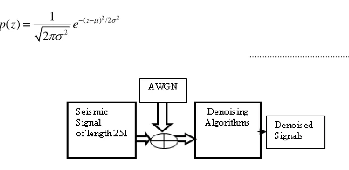
Pdf of Gaussian distribution is
...( 1)
Figure 1 White Gaussian Noise model
In this model, Seismic signal of length 251 are generated and AWG Noise with mean=0 and =1.0 is added to the seismic signal. Noise is varied in 2dB steps from -4dB to +16dB. Noisy Seismic signal is then denoised using Wavelet Transform based algorithms and results are compared for performance using SMSE criterion.
Model 2) Flicker Noise or Pink color noise Model:
The flicker noise is sometimes used to refer to pink noise, although this is more properly applied only to its occurrence in electronic devices. Pink noise or 1⁄f noise is a signal or process with a frequency spectrum such that the power spectral density (energy or power per Hz) is inversely proportional to the frequency of the signal. In pink noise, each octave (halving/doubling in frequency) carries an equal amount of noise power. The name arises from the pink appearance of visible light with this power spectrum.
2 2
( ) /2
2
1
( )
2
z
p z
e
Figure 2 Ficker or pink noise model
In this model, Seismic signal of length 251 are generated and Pink color Noise '1/f' is added to the Seismic signal. Noise is varied in 2dB steps from -4 dB to +16dB . Noisy Seismic signal is then denoised using Wavelet Transform based algorithms and results are compared for performance using SMSE criterion.
Model 3) Impulse Noise Model:
Impulse noise or spike noise also called salt-and pepper noise is usually caused by timing errors in the process of digitization, faulty memory locations, malfunctioning of pixel elements in Camera sensors. Impulse noise of equal height impulses is called salt-and pepper noise and there are only two possible values exist that is a and b the probability of each is less than 0.2.Impulse noise of un equal height impulses is called random values impulse noise is used in this model. The probability density function of impulse noise is
... (2)
Figure 3 Impulse noise model
In this model, Seismic signal of length 251 are generated and Impulse Noise with mean=0 and =1.0 is added to the Seismic signal. Noise is varied in 2dB steps from -4dB to +16dB .Noisy Seismic signal is then denoised using Wavelet Transform based algorithms and results are compared for performance using SMSE criterion.
Model 4) Rayleigh Noise Model:
( ) 0
a
b
P for z a
p z P for z b
otherwise
Figure 4 Rayleigh noise model
Rayleigh fading is viewed as a reasonable model for tropospheric and ionospheric signal propagation as well as the effect of heavily built-up urban environments on radio signals. Rayleigh fading is most applicable when there is no dominant propagation along a line of sight between the transmitter and receiver. How rapidly the channel fades will be affected by how fast the receiver and/or transmitter are moving. The probability density function of the Rayleigh distribution is
... ( 3)
In this model, In this model, Seismic signal of length 251 are generated and Rayleigh Noise with mean=0 and =1.0 is added to the Seismic signal. Noise is varied in 2dB steps from -4 dB to +16dB .Noisy Seismic signal is then denoised using Wavelet Transform based algorithms and results are compared for performance using SMSE criterion.
III. WAVELET ANALYSIS
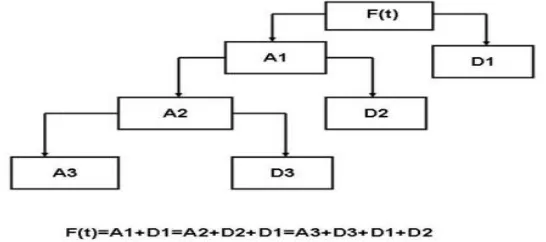
The wavelet transform is very useful tool in the analysis of non stationary signals such as the reflection seismic signals. The theory and methods of wavelet analysis are detailed in books[3],[4].In this paper, discrete wavelet analysis is used instead of the continuous wavelet analysis. The discrete wavelet analysis is based on the concept of Multi-resolution analysis (MRA) introduced by Mallat [5].With the MRA, a signal is decomposed recursively into sum of details and approximations at different levels of resolution as shown in Figure 5
The details represent the high frequency components while the approximations represent the low frequency components of the signal. The decomposition algorithm is fully recursive. At each stage of MRA the signal is passed through a High pass filter called scaling filter, denoted as G and a Low pass filter called the wavelet filter, denoted as H.These filters are quadrature mirror filters that satisfy the orthogonality conditions; HG*=GH*=0 and H*H+G*G=I ; where I is the identity operator. The filters H and G are the decomposition filters , while the filters H* and G* are the reconstruction filters.
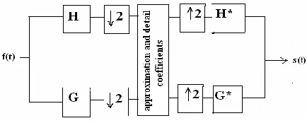
The coefficients of the filters H and G depend on the particular wavelet used for the decomposition [6].The process of decomposing a signal f(t) and reconstructing the approximations Ai and Di is shown in Figure 6.
Figure 6. The process of decomposition and reconstruction of approximations (Ai) and details (Di) (level i). Symbols 2 2 represent dyadic down-sampling and up-sampling.
As shown in figure 6, the discrete wavelet transform (DWT) analyzes the signal at different frequency bands and with different resolutions by decomposing the signal in to coarse approximation and detail information. The approximation components are obtained by passing the signal through the low pass filter H, which removes the high frequency components. At this stage, the resolution is halved but the scale remains unchanged .Then, the signal is sub-sampled, thereby removing half the redundant samples. It should be noted that this process does not affect the resolution but affects the scale, which is doubled. Similarly the detailed coefficients are obtained by passing the signal through the high pass filter G. his constitutes one level of de-composition. The wavelet coefficients thus obtained can then be used for the purposes of signal de-noising and compression [7].
A. Threshold Algorithms
To denoise a signal using wavelet transforms the detail coefficients are thresholded[8] . The simplest threshold technique is the hard threshold, where the new values of the details coefficients d(t) are found according to the following:
--- ( 4) Where d(t) are detailed coefficients and is the threshold
Another method of threshold is the soft threshold, where the new details coefficients are given by the following:
...,...--(5)
The threshold can be estimated using different threshold estimating algorithms and widely used Universal Threshold is as follows:
.---( 6)
Hard threshold can be described as the usual process of setting to zero the elements whose absolute values are lower than the threshold. Soft threshold is an extension of hard threshold, first setting to zero the elements whose absolute values are lower than the threshold, and then shrinking the nonzero coefficients towards 0. Threshold selection rules and algorithms are described in next section.
I. Universal Threshold
This type of global thresholding method was proposed by Donoho and Johnstone. This is also called Universal threshold method. The threshold value is given in equation (6) , where N is the number of data points, and ‘σ’ is an estimate of the noise level. Donoho and Johnstone proposed an estimate of σ that is based only on the empirical wavelet coefficients at the highest resolution level (j -1) because they consist most of noise. Most of the function information except the finest details is in lower level coefficients. The median of absolute deviation (MAD) estimator is expressed in equation (6) as
median( Wj-1,k-median(Wj-1,k ) /0.
6475
... … (7)The universal thresholding removes the noise efficiently. The fitted regression curve is often very smooth and hence visually appealing. If z1... zn represent the wavelet coefficients of the noise with idd N (0, σ2), then it is expressed in
equation (7) as
...………..…(8) This means that the probability of all noise being shrunk to zero is very high for large samples.
.
B DENOISED SIGNAL RECONSTRUCTION
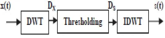
Because of the amplitude based muting (based on thresholds) wavelet-transform based filters are in general nonlinear and can be readily applied to non-stationary reflection signals. Wavelet filters are efficient for filtering several types of noise in seismic data at the same time. Reconstruction or synthesis is the process of assembling those components back into the signal .The mathematical manipulation that affects synthesis is called: the inverse
discrete wavelet transforms (IDWT).In order to get the de-noised signal, the new details coefficients, , are used
in signal construction process instead of original coefficients d(t). The de-noised procedure is summarized in Figure 7.
Figure 7. DWT de-noising procedure.
IV. MODIFIED DENOISING APPROACH
A. Disadvantages of Wavelet Denoising
The general wavelet de-nosing procedure starts with first selection of a wavelet that may not match varying nature of signals resulting a drawback. However , to some extent this drawback can be minimized based on eyeball inspection of the signal with noise , or it can be selected based on correlation γ between the signal of interest.
The second disadvantage wavelet denoising is decomposition of signal in to coefficients based on fixed level irrespective of Signal SNR is high or low. Thus the decomposition level is non adaptive.
B. The Hurst Coefficient
In this section, we propose a new denoising approach. This approach is based on Hurst coefficient proposed by H. E. Hurst [9] for denoising use. The Hurst exponent provides a measure for long term memory and fractality of a time series. Since it is robust with few assumptions about underlying system, it has broad applicability for time series analysis. The values of the Hurst exponent range between 0 and 1.Based on the Hurst exponent value H, a time series can be classified into three categories. (1) H=0.5 indicates a random series. (2) 0<H<0.5 indicates an anti-persistent series or noise dominated (3) 0.5<H<1 indicates a anti-persistent series. An anti anti-persistent series has a characteristic of “mean-reverting”, which means an up value is more likely followed by a down value, and vice versa. The strength of “mean reverting” increases as H approaches 0.0. A persistent series is trend reinforcing, which means the direction ( up or down compared to the last value) of the next value is more likely the same as current value. The strength of trend increases as H approaches 1.0.
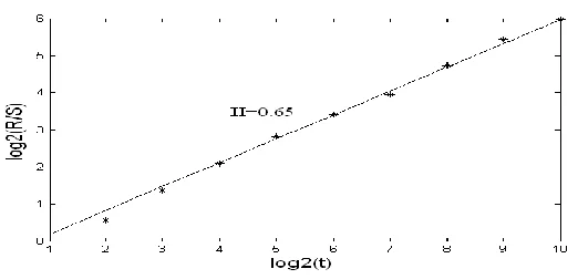
The best-known method to estimate the Hurst exponent is R/S analysis. It was proposed by Mandelbrot and Wallis [10], based on the previous work of Hurst .
The procedure is as follows.
The time series of length L has to be divided into d sub series (Zi,m) of length n, and for each sub series m = 1, . . , d. Then,
1. It is necessary to find the mean (Em) and the standard deviation (Sm) of the sub series (Zi,m).
2. The data of the sub series (Zi,m) has to be normalized by subtracting the sample mean Xi,m = Zi,m − Em for i =1, .n
3. Create the cumulative time series Yi,m =
1
i j
Xj,m for i = 1, . . . , n.4. Find range Rm = max{Y1,m ,.. Yn,m } -min {Y 1,m,..Y n,m}
5. Rescale the range (Rm/Sm).
6. Calculate the mean value (R/S)n of the rescaled range for all sub series of length n.
Considering that the R/S statistic asymptotically follows the relation (R/S)n ≈ c nH, the value of H can be obtained
by running a simple linear regression over a sample increasing time horizons.
log (R/S)n = log c + H log n. ………. (9)
Figure 8 An example of R/S analysis
C. Modified Threshold Method
the noisy signal.
However, we find the thresholds decrease so slowly from the first to the last part of the signal may get lost from some signal-dominated detail coefficients after thresholding. Therefore , we should first find the detail coefficients which are dominated by the noise and the ones dominated by the signal .Then we apply the universal threshold to the noise dominated detail coefficients, and another estimating threshold method which is able to decrease faster to the signal dominated detail coefficients..
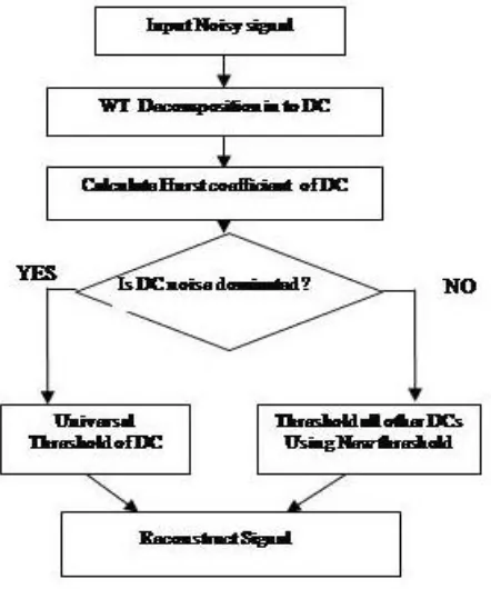
The modified denoising approach consists of three key steps: firstly , find the detail coefficients dominated by noise and threshold them separately; secondly, compute the thresholds of other detail coefficients using a new estimating threshold which is able to decrease faster; lastly, apply the thresholding technique to each detail coefficient, and then reconstruct the signal by adding the thresholded detail coefficients. Detail explanations are :
1) Find the detail coefficients dominated by the noise.
We have introduced Hurst exponent method to find the noise dominated detail coefficients.Based on the Hurst exponent value H, a time series can be classified into an anti-persistent series if its H value is between 0 and less than 0.5.Therefore,in practice , in deciding whether the detail coefficient is noise dominated or not is judged by its Hurst coefficient value H. Then we use the Universal threshold method to estimate threshold level and threshold each noise dominated detail coefficients.
2) Get the thresholds of the other Detail Coefficients.
We have to find another estimation method to get the thresholds of the signal dominated detail coefficients. Since the estimation of Universal threshold decrease slowly or more or less remain constant, we need one which can decrease faster for signal dominated detail coefficients.
First, through studying the Universal threshold
...…….. (10) Thr i =ө =C√(V/β) .
-i
. 2log N ... ……(11) V is the energy and β ,
are the parameters [11] and equal to 0.179 and 2.01 respectively when the noise is white Gaussian noise.Removing constant term and substituting
≈ 2Thr i ( new)
(√2) -i... ………..(12)
In order to make this threshold decreased faster, the form of new modified threshold that we are proposing will be an exponential function. and we set
Thr i ( new)
-i , i=1,2,3,4 ...……….(13)The new threshold function needs to be proportional to the threshold of the last noise dominated detail coefficient ‘k’.Thus the expression of the threshold is set as:
Thr i ( new) = Thr k / i-k , i=k+1,……K …..(14)
2.4 for noisy signal denoising
Thr i ( new) = Thr k / 2 i-k
, i = k+1…K. …..(15)
Figure 9 Comparison of Two threshold methods.
3) Use the estimated thresholds to each detail coefficient
Now the thresholds of each detail coefficient is being determined , threshold the signal dominated detail coefficients and then reconstruct the signal.
Figure 10. New WT modified threshold denoising approach Scheme
V. EXPERIMENTAL RESULTS
SMSE=1/N 1 N
j
E {|x, - Xj |2} ... (16)Where xj is the source signal or the noise free signal, Xj is estimated signal, and N is sample number of the signal.
The performance is better when the value of SMSE is smaller.
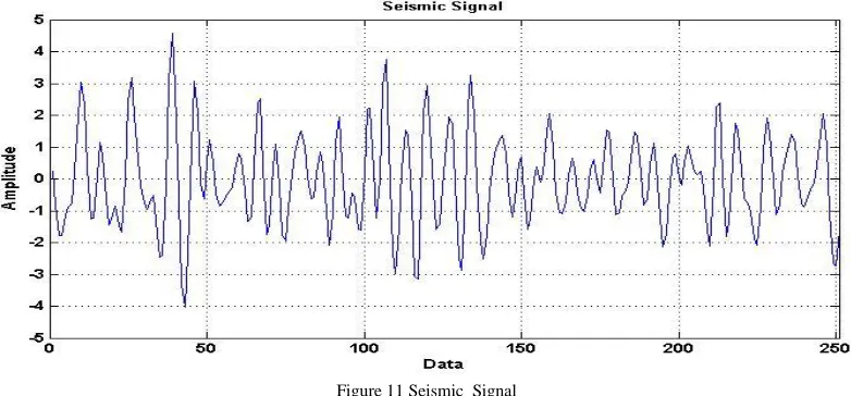
Figure 11 Seismic Signal
We performed numerical simulation of Seismic test signal using MATLAB as shown in figure 11. The sample size of the signals is N=251.The parameters of WT are set as the basis function is “sym7” and the number of decomposition levels is 12. In order to compare the effect of Universal threshold algorithm with new modified threshold approach in denoising of noise components we have constructed Four kinds of stochastic models 1) White Gaussian Noise model 2) Flicker noise model 3)Impulse noise model and 4) Rayleigh noise model.
Figure 12 shows the SMSE comparison for White Gaussian Noise model. The new modified approach is very efficient and outperforms universal threshold algorithm. in the presence of strong white Gaussian noise. Comparison of two types of threshold algorithms shows that both threshold algorithms could reduce the distribution of white Gaussian noise up to SNR of 16 dB with modified threshold algorithm performing better. For SNR from 2dB to -4dB the performance of each algorithm differed with steep rise in their SMSE .Modified threshold algorithm performing better in the cases where the signal SNR is low.
Figure 12 Denoising performance of threshold algorithms for White gaussian noise
Table 1: SMSE values of Universal and Modified Threshold algorithms for White gaussian noise
Universal 3.2457 2.0548 1.3858 1.1891 1.204 1.2343 1.2848 1.2922 1.2527 1.2526 1.2374
Figures 13,14 and 15 show the comparison of threshold algorithms for the noise model 2,3 and 4 respectively.It can be seen by comparison of figures 13, 14 , and 15 that there is significant effect of threshold algorithms in denoising of noise models of Flicker noise,Impulse noise and Raleigh noise.
Figure 13 Denoising performance of threshold algorithms for flicker noise
Table 2: SMSE values of Universal and Modified Threshold algorithms for White gaussian noise
Universal 4.5534 3.2227 2.4485 1.8693 1.5924 1.4875 1.4553 1.4109 1.2958 1.2806 1.2844 Modified 3.3374 2.3178 1.7373 1.3978 1.0449 0.9169 0.8507 0.8162 0.7974 0.7875 0.7827
In model 2 we can observe the denoising performance is poor compared to model 1 with modified threshold approach performing better. The performnace difference between them remained same from 16dB SNR to -4dB SNR with modified threshold performing better . Both algorithms perform poor in the range from 4dB to -4dB .
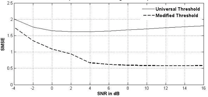
Figure 14 Denoising performance of threshold algorithms for impulse noise
Universal 2.0086 1.7616 1.652 1.6173 1.6207 1.6446 1.6767 1.7104 1.7425 1.7712 1.7961 Modified 1.7555 1.3443 1.0901 0.9393 0.6683 0.6172 0.5935 0.5829 0.5798 0.5809 0.5838
In noise models 3 and 4 , we can observe the the performance of Universal Threshold algorithm differ from that of modified threshold algorithm through out the SNR range starting from 16dB to -4dB.In model 3 the worst case SMSE is 1.75 for modified threshold compared to 2 of Universal Threshold algorithm.
In noise model 4, Modified threshold performed poor in the SNR range starting from -2dB to -4dB. The performnace of modified threshold algorithm is better for high SNR compared to low SNR.
Figure 15 Denoising performance of threshold algorithms for Rayleigh noise
Table 4 : SMSE values of Universal and Modified Threshold algorithms for Rayleigh noise
Universal 6.9668 4.5237 3.0441 2.3975 1.8211 1.4649 1.2747 1.1682 1.1121 1.0857 1.0764 Modified 6.5708 4.4464 3.1981 2.4778 2.0711 1.8554 1.7476 1.7061 1.701 1.7141 1.7354
VI. CONCLUSIONS
In this paper we applied two thresholding algorithms, Universal Threshold and modified Threshold algorithm in an aim to impact of thresholding in denoising of Seismic signals. In order to compare the effect of them in denoising of noise components we have constructed four kinds of stochastic models: the white gaussian noise model (1), the Flicker noise model(2),the Impulse noise model (3) and Rayleigh noise model (4). SMSE criterion is used for performance measurement.The results are:
1. In model (1) and (2) , both threshold algorithms could reduce the distribution of white gaussian noise and Flicker noise in different degree.New modified threshold algorithm could remove almost complete noise for SNR from 16dB to -4dB while algorithms could remove noise reasonably for SNR from 16dB to 0dB then the denoising performance exponentially degraded for SNR from 4 dB to -4 dB .
2. In model (3) and (4) ,from Figures 14 and 15, both threshold algorithms could reduce the distribution of Impulse and Rayleigh noise in different levels with new modified threshold algorithm performing better. Universal algorithm could not remove impulse noise efficiently for SNR starting from 16dB to 0 dB and the performnace exponentially degraded for SNR between 0 dB and -4dB.Modified algorithm performed better compared to Universal algorithm.In the case of Rayleigh noise both algorithms performed more or less same with modified algorithm performing little poor compared Universal in the SNR range from -2dB to -4dB.
REFERENCES
[2] Priyanka Kamboj and Versha Rani, A Brief study of Various noise models and Filtering Techniques, Journal of Global Research in Computer Science, Vol 4,No4, April 2013.
[3] Chui C K An introduction to wavelet, Academic Press,1992
[4] Teolis A., Computational Signal Processing with Wavelets, Brikhauser, Boston 1998.
[5] Mallat S."A theory of multiresolution signal decomposition:The wavelet Representation, IEEE Trans. Pattern Anal. Machine Intelligence,pp/674-693,1989.
[6] Roman W.,"Determination of P phase arrival in low amplitude seismic signals from coalmines with wavelets"
[7] Sid-Ali Ouadfeul, Leila Aliouane, Mohamed Hamoudi, Amar Boudella2 and Said Eladj., "1D Wavelet Transform and Geosciences [8] Donoho,D.L (1995),"De-noising by Soft-thresholding" IEEE Trans.on Inf.Theory 41,3 pp 613-627
[9] H.E. Hurst, Long-term storage of reservoirs: an experimental study, Transactions of the American society of civil engineers, 116, 1951, 770-799.
[10] Bo Qian Khaled Rasheed, Hurst Exponent and Financial Market Predictability, University of Georgia-USA