INTERNATIONAL JOURNAL OF SCIENTIFIC & TECHNOLOGY RESEARCH VO
Survival Analysis By Using
With
Abstract: Cox regression model is one of the models can be used in analyzing survival data and we
variables and their survival time, so the cox regression is semi parametric model that consist two parts, the first part is n parametric part (eβ
) where β is the vector of unknown parameters, ( one of censoring was taken from hospital with left-censored
distribution of survival time is unknown. Selecting cox regression model as the best model to analysis data by checking the a model once graphically by using Kaplan–Meier estimator
by using (partial likelihood) method and test the model parameter by using (Wald) test which shown that only two parameters(treatment and anemi status) are effect on survival time.
Index Terms: Cox regression model, survival time, with
estimator to estimating the survival function and partial likelihood) method with (Wald) test. ——————————
1
I
NTRODUCTIONSurvival analysis is a branch of statistics which
analysis of time to events, such as death in biological organisms and failure in mechanical systems. This topi called reliability theory or reliability analysis in engineering, and duration analysis or duration modeling in
event history analysis in sociology. Survival analysis attempts to analysis the proportion of a population which will survive past a certain time. The Cox regression model (Cox, 1972) is the most popular method in regression analysis for censored survival data. However, due to the very high dimensional space of the predictors, the standard maximum Cox partial likelihood method cannot be applied directly to obtain the parameter estimates. To deal with the problem of co linearity, the most popular approach is to use the penalized partial likelihood which was proposed by Tibshirani (1995) and is called the least absolute shrinkage and selection operator (Lasso) estimation. In the case of biological survival,
unambiguous, but for mechanical reliability, failure
well-defined, for there may well be mechanical systems in which failure is partial, a matter of degree, or not otherwise localized in time. Even in biological problems, some events (for example, heart attack or other organ failure). More generally, survival analysis involves the modeling of time to event data; in this context, death or failure is considered an "event" in the survival analysis literature traditionally only a single event occurs for each subject, after which the organism or mechanism is dead or broken. The study of recurring events is relevant in systems reliability, and in many areas of social sciences and medical research.The survival function, also known as a survivor function or reliability function, is a property of any random variable that maps a set of events, usually associated with mortality or failure of some system, the term survival function is used in a broader range of applications, including human mortality.
__________________________________
• Dr. Monem A. Mohammed University of Sulamani Email: [email protected]
CHNOLOGY RESEARCH VOLUME 3, ISSUE 11, NOVEMBER 2014
Analysis By Using Cox Regression Model
With Application
Dr. Monem A. Mohammed
Cox regression model is one of the models can be used in analyzing survival data and we can detect relationship between the explanatory variables and their survival time, so the cox regression is semi parametric model that consist two parts, the first part is n
is the vector of unknown parameters, (z) is the vector of explanatory variable. The data which used in this study is type
censored data, testing distribution of survival time by using goodness of test and we find the distribution of survival time is unknown. Selecting cox regression model as the best model to analysis data by checking the a
Meier estimator to estimating the survival function from lifetime data of patients, We estimated the
likelihood) method and test the model parameter by using (Wald) test which shown that only two parameters(treatment and anemi Cox regression model, survival time, with left-censored data, testing distribution of survival time by using goodness of fit,
partial likelihood) method with (Wald) test.
————————————————————
which deals with analysis of time to events, such as death in biological organisms and failure in mechanical systems. This topic is or reliability analysis in engineering, and duration analysis or duration modeling in economics or . Survival analysis attempts which will survive past a certain time. The Cox regression model (Cox, 1972) is the most popular method in regression analysis for censored survival data. However, due to the very high dimensional space of the predictors, the standard maximum Cox partial ikelihood method cannot be applied directly to obtain the parameter estimates. To deal with the problem of co linearity, the most popular approach is to use the penalized partial likelihood which was proposed by Tibshirani (1995) and is solute shrinkage and selection operator (Lasso) estimation. In the case of biological survival, death is failure may not be defined, for there may well be mechanical systems in which failure is partial, a matter of degree, or not otherwise problems, some events or other organ failure). More generally, survival analysis involves the modeling of time to ontext, death or failure is considered an "event" in the survival analysis literature traditionally only a single event occurs for each subject, after which the organism or mechanism is dead or broken. The study of recurring events , and in many areas of social sciences and medical research.The survival function, also known as a survivor function or reliability function, is a f any random variable that maps a set of events, usually associated with mortality or failure of some system, the term survival function is used in a broader range of
2
DEFINITIONS:
Let (T) be a continuous random variable with distribution function F(t) on the interval [0, function is:
2.1 Properties:
Every survival function S(t) is monotonically decreasing S(u) ≤ S(t) for all . The time
origin, typically the beginning of a study or the start of operation of some system. S(0) is commonly unity but can be less to represent the probability
immediately upon operation.
3 Lifetime distribution function and event
density:
The lifetime distribution function, conventionally denoted defined as the complement of the survival function,
If (F ) is differentiable then the derivative, which is the density function of the lifetime distribution, is conventionally denoted ( f),
The function (f ) is sometimes called the the rate of death
4 Hazard function and cumulative
function:
The hazard function, denoted (λ), is defined as the event rate at time (t) Conditional on survival until time (
T≥t),
λ t Lim →
∖
! "
#" "
The hazard function must be non
integral over must be infinite, but is not otherwise __________________________________
Dr. Monem A. Mohammed University of Sulamani-
VEMBER 2014 ISSN 2277-8616
314
Regression Model
can detect relationship between the explanatory variables and their survival time, so the cox regression is semi parametric model that consist two parts, the first part is nonparametric (λt and other is ) is the vector of explanatory variable. The data which used in this study is type data, testing distribution of survival time by using goodness of test and we find the distribution of survival time is unknown. Selecting cox regression model as the best model to analysis data by checking the assumption Cox regression from lifetime data of patients, We estimated the parameters likelihood) method and test the model parameter by using (Wald) test which shown that only two parameters(treatment and anemia tion of survival time by using goodness of fit, Kaplan–Meier
Let (T) be a continuous random variable with cumulative F(t) on the interval [0,∞). Its survival
$ %&'&∞ ( # )
monotonically decreasing, i.e. time, t = 0, represents some origin, typically the beginning of a study or the start of operation of some system. S(0) is commonly unity but can be probability that the system fails
Lifetime distribution function and event
The lifetime distribution function, conventionally denoted F, is defined as the complement of the survival function,
) is differentiable then the derivative, which is the density function of the lifetime distribution, is conventionally denoted
) is sometimes called the event density; it is
Hazard function and cumulative hazard
), is defined as the event rate ) Conditional on survival until time (t) or later (that is,
constrained; it may be increasing or decreasing, non monotonic, or discontinuous, also hazard function c alternatively be represented in terms of the
hazard function, denoted( ):
so transposing signs and exponentiation
or differentiating (with the chain rule)
The name "cumulative hazard function" is derived from the fact that:
Which is the “accumulation” of the hazard over time?
definition of , we see that it increases without bound as (t ) tends to infinity (assuming that S(t) tends to zero). This implies that must not decrease too quickly, since, by definition, the cumulative hazard has to diverge. For example, is not the hazard function of any survival distribution, because its integral converges to (1).
4 Types of data:
4.1 Complete data: that is meaning the values of each sample unit is observed or known.
4.2 Censored data: that is mean a form of death dates of a subject are known, in which case the lifetime is known. known only that the date of death is after some date, this is called right censoring. Right censoring will occur for those subjects whose birth date is known but who are still alive when they are lost to follow-up or when the study ends.
lifetime is known to be less than certain duration, the lifetime is said to be left-censored. It may also happen that subjects with a lifetime less than some threshold may not be observed at all: this is called truncation. We generally encounter right censored data. Left-censored data can occur when a person's survival time becomes incomplete on the left side of the follow up period for the person. As an example, we may follow up a patient for any infectious disorder from the time of his or her being tested positive for the infection. We may never know the exact time of exposure to the infectious agent.
5 Multiple Regression model:
A Multiple Regression model is a model with a multiple explanatory variables and we can represent as the follows:
Y βZ +e
constrained; it may be increasing or decreasing, non-monotonic, or discontinuous, also hazard function can alternatively be represented in terms of the cumulative
The name "cumulative hazard function" is derived from the fact
Which is the “accumulation” of the hazard over time? From the , we see that it increases without bound as ) tends to zero). This must not decrease too quickly, since, by definition, the cumulative hazard has to diverge. For example, is not the hazard function of any survival distribution, because its integral converges to (1).
the values of each
that is mean a form of death dates of a subject are known, in which case the lifetime is known. If it is known only that the date of death is after some date, this is censoring. Right censoring will occur for those subjects whose birth date is known but who are still alive when up or when the study ends. If a subject's lifetime is known to be less than certain duration, the lifetime is censored. It may also happen that subjects with a lifetime less than some threshold may not be observed at all: . We generally encounter right-censored data can occur when a person's
incomplete on the left side of the follow-up period for the person. As an example, we may follow follow-up a patient for any infectious disorder from the time of his or her being tested positive for the infection. We may never know the
he infectious agent.
A Multiple Regression model is a model with a multiple explanatory variables and we can represent as the follows:
Where Y is the response variable, (
parameters, (Z) is a non singular matrix of explanatory variables, so the Properties of multiple regression model it is important to make sure that the underlying assumptions hold. Plotting residuals versus the (Z) values and ot
diagnostics are useful to check the normality of data.
5.1 Proportional Hazards Models:
These models an important model which usually associated with mortality or failure of some system, so we can find a combined model with survival time and
follows:
λt; z λt exp (β Z … ( 1)
Where λ-t, z/ is an arbitrary hazard rate function at time (t) for an individual with covariates Z
unspecified base- line hazard function for continuous (t), the regression coefficients, The density function, S(
S-t; Z/ -t; z/S-t; Z/
= exp (-1λuexpβ Zdu
The regression coefficientsβ
assumptions made about the hazard function then one would maximize the likelihood functions and would consider contributions made to the hazard rate by censored data. are some Proportional Hazards Models for survival data as follows:
5.2 Exponential regression model:
In this model assume that (survival time) have exponential distribution with (pdf):
f( t ∖z= 7
λ exp(
8
λ , t > 0 … (3)
Where (λz is aconstsnt hazard function λz Et ∖z= exp(β z
which depend on regression parameters (
variables (z).Therefore the survival functions as follows: S( t ∖z= exp{-(
BCDβ E … (4)
Then the likelihood function is the product of the likelihood of each datum as follows:
L(β, t, z= πFG7H ( 7
BCDβ I exp (
5.3WIBULLL REGRESSION MODEL:
In this model assume that (survival time) have continuous probability wibull distribution with (pdf):
f( t ∖z= BCDαβ ( BCDβ α87expJ 8
BCD
The hazard function of wibulll regression model can take
315
is the response variable, (β ) is the vector of unknown parameters, (Z) is a non singular matrix of explanatory Properties of multiple regression model it is important to make sure that the underlying assumptions hold. Plotting residuals versus the (Z) values and other residual diagnostics are useful to check the normality of data.
1 Proportional Hazards Models:
These models an important model which usually associated with mortality or failure of some system, so we can find a combined model with survival time and hazard function as
… ( 1)
is an arbitrary hazard rate function at time (t) for
Z ), λt is an arbitrary line hazard function for continuous (t), β is on coefficients, The density function, S(t) is:
/
du … (2)
may be estimated with assumptions made about the hazard function then one would maximize the likelihood functions and would consider contributions made to the hazard rate by censored data. There are some Proportional Hazards Models for survival data as
2 Exponential regression model:
In this model assume that (survival time) have exponential
… (3)
function with
regression parameters (β and explanatory ).Therefore the survival functions as follows:
… (4)
Then the likelihood function is the product of the likelihood of
exp ( 8
BCDβ I) … (5)
:
In this model assume that (survival time) have continuous wibull distribution with (pdf):
8 β E
α , t > 0 , α > 0 … (6)
INTERNATIONAL JOURNAL OF SCIENTIFIC & TECHNOLOGY RESEARCH VOLUME 3, ISSUE 11, NOVEMBER 2014 ISSN 2277-8616
316
follows formula:
λ-t ∖ z/ α BCDβ (
BCDβ
α87 … (7)
Then, the survival function has the following formula: S ( t ∖z= expJ 8
BCDβ E
α … (8)
So, the likelihood function can take the following: L (β, t, z= πFG7H {[BCDααβLM ]α exp(
BCDβ
α }{exp (
BCDβ
α} … (9)
6 Co
P
,Q
Regression Model:
This model one of important models published by (D.R. Cox in 1972) and is one of most frequently articles in statistics and medicine, which usually associated with mortality or failure of some system, he suggested that model depend on (hazard rate) in time (t), as the follows:
λt; z λt exp(β Z = λtexp (∑DFG7βFZF … (10)
λt : Initial hazard function when all values of (Z 0.
β : are unknown’s regression coefficients. (Z): is the p-dimensional vector of covariates. We can write survival function of (10) as follows:
S-t; Z/ JStE exp (∑DFG7βFZF … (11)
Where exp (∑DFG7βFZF is the proportional hazard function. But, Cox model is a semi- parametric model with free distribution. So, the estimation problem for (β) is the same under any transform. Only the rank statistic r (.) can carry information about (β) when λis completely unknown. It follows that the rank statistic is marginally sufficient to estimate (β). To apply the rank statistic to get inferences about (β), one would use the marginal distribution of the ranks and the marginal likelihood.
7 Marginal Likelihood:
Suppose (n)individuals are observed to fail at times ( TF , i = 1,… , n), with corresponding covariates (z7 ,… , zH). Assume that all failure times are distinct, i.e. no two people (or more) fail or are censored at the same time. The order statistic is defined to be O (t) = [T (1); T(2), …, T(n)] and refers to the T is being ordered increasingly i.e. (T(1) < T(2) < …< T(n)). The rank statistic is defined to be r (t) = [(1), (2), …, (n)] and refers to the label attached to the order. To apply the rank statistic to get inferences about (β) one would use the marginal distribution of the ranks and the marginal likelihood. The marginal likelihood is proportional to the probability that the rank vector is observed, i.e.
Pr(r, β) = pr{r = [1, 2, 3… n] ; β}=
1 1 … 1∞ 7∞ H87∞ πFG7H ftF, zFdtH… dt7
and we find : Pr(r, β) = \ UPV∑ZX[(WXY
X[(
Z J∑ UPVW]YE
]∈_ X … (12)
Where RtF is R(t) = {i: T(i) ≥ t } the risk set at time T(i), that is the group of individuals (i ) that are under observation at time (t),
i.e., T (i)) = {(i), (i + 1) ... (n)}.
To deal with censored data one must modify this last argument. If censoring Takes place, the group then acts transitively on the censoring time and the invariant in the sample space is the first (k) rank variables, i.e. (1), (2) … (k). For example, if we observe the following failures: T7=110,
Ta70, Tb 64∗, Tf90, (n =4) with (12) symbolizing a
censored observation. Then the following rank statistics are possible:
[3, 2, 4, 1], [2, 3, 4, 1], [2, 4, 3, 1], [2, 4, 1, 3].
Suppose (k) items are observed, labeled (1), (2), …, (k), and have failure time {T(1), T(2), … , T(n)} with corresponding covariates {z7 ,… , zH }. Suppose further that (
mF observations with covariates {zF7 ,… , zFgIE are censored in
the ith interval [ TF, TF7; i = 1, 2,…, k, where T(0) = 0 and T(k+1) = ∞. The marginal likelihood of (β) is computed as the probability that the rank statistic should be one of the possibilities, which is then the sum of the large number of terms as in equation (20). The possible rank vectors can be characterized as:
T7< Ta< …< Th
And TF< TF7, TFa , …< TFg <TFgI , i=0, 1,2, …, k. … (13)
Where TF7, …, TFg ) (the unobserved failure times) associated with the censored individuals in [TF, …, TF7). So, the event (TF) has the conditional probability:
h(TF) = exp[ - ∑ giG7I β ZFi 1Iλudu]
, i = 1,2,…,k … (14)
So, the Probability marginal likelihood is proportional to the probability of the event (14) is:
1 1 … 1∞ 7∞ h87∞ πFG7H ftF, zFλtFdth… dt7 .
Now, we can find: Pr(r, β) = \ UPV∑jX[(WXY
X[(
j J∑ UPVW]YE
]∈_ X … (15)
8 Partial Likelihood:
Cox (1975) has shown that this partial log-likelihood can be treated as an ordinary log-likelihood to derive valid (partial) MLEs of (β). Therefore we can estimate hazard ratios and confidence intervals using maximum likelihood techniques. The only difference is that these estimates are based on the partial as opposed to the full likelihood. The partial likelihood is valid when there are no ties in the data set that is no two subjects have the same event time, if there are ties in the data set, the true partial log-likelihood function involves permutations and can be time-consuming to compute. Then, to study (Cox) model which have the following hazard function:
λ-t ∖ z/ λtexp (β z with T7< Ta< …< TH
317
models in which the response variable is time. However, computing the likelihood function (needed for fitting parameters or making other kinds of inferences) is complicated by the censoring. So, the likelihood function can take the following:
Lβ,λt, t, z
πFG7H JλtF exp β zEδIexp J# $λ
uexp β zduE I
πFG7H BCDkβ lIm
J∑n∈o-pI/BCDβ lnE∑q∈rIλtexp kβ ZqmπFG7
H S
tFexp kβ zm.. 16
Where St exp (- 1λuduThe previous likelihood equations are special cases of (16). Equation (16) can be approximated by:
L(β,t, z= πFG7H UPVkY WXm J∑]∈_- X/UPVYW]E
The maximum likelihood estimate of (β ) is (βu ) and can be obtained as a solution to the system of the following equations:
v wxy V]Y, ,z
v YX = ∑ J ZF
h FG7 #
∑]∈_- X/UPVkY W]mW]X
∑]∈_- X/UPVY W] }
and similarly one can get: v{wxy V]Y, ,z
v YX v Y| =
∑ Jj XG(
∑]∈_- X/UPVkY W]mW]XW]|
∑]∈_- X/UPVY W] #
∑]∈_- X/UPVkY W]mW]X
∑]∈_- X/UPVY W] ∗
∑]∈_- X/UPVkY W]mW]|
∑]∈_- X/UPVY W] }
… (17) Where (j = 1, 2, 3 … S)
9 Testing data for goodness:
There many formulas using to testing for goodness data as follows:
9.1 Log Rank Test:
The log rank test is a popular test to test the null hypothesis of no difference in survival between two or more independent groups.. Survival curves are estimated for each group, considered separately, using the Kaplan-Meier method and compared statistically using the log rank test. The log rank test compares the observed number of events in each group to what would be expected if the null hypothesis were true (i.e. if the survival curves were identical). H0: The two survival curves are identical versus H1: The two survival curves are not identical with (α=0.05). The log rank statistic is approximately distributed as a chi-square test statistic, as follows:
Xa =∑ ~I8 I
I
H
FG7 … (18) 9.2 Score test statistic:
There are many statistical testing for proportional hazard assumption, one of them is the (Score test statistics) which used to test how effect the covariate vector for proportional hazard in time (t), let the state of unit from life to death can putting in the following model:
λ-t ∖ z/ λt exp {Z β+γtE if t ϵI … (19)
for each time with sequencings (I), therefore we can give the test hypothesis as follows:
H: γ7γa ⋯ γD 0 Versus
H7: at least one of them not equal to zero
With following test statistics: S = UV87 U … (20)
Where {U} represent the vector of derivatives of log l likelihood under H and partial likelihood for vector (β and
(V) = - { v{wxy V]Y, ,z
v YX v Y| E.
So, the score test close to chi- square distribution with (p) degree of freedom.
9.3 Wald Test:
Another common way to test for the individual hazard ratio is based on Wald test which is testing whether the individual hazard coefficient is zero or not with H: βi 0.
The Wald test ( Wi = { " β βE
a … (21)
10 Experimental Part:
10.1 Descriptiondata:
In this research we use a real data of (Nankelly - hospital) in Arbeil city- Iraq, we have (72) patients with Leukemia disease from (1-9-2013) to (31-12-2013). We study the following variables:
T: Survival Time
7: The age of patient in first visit hospital
a: The gender of patient takes (1 for male and 2 for female)
b: Disease type takes follow:
1- Acute myeloid leukemia /AML 2- Acute Lymphocytic leukemia / ALL 3- Chronic mylelogenous leukemia/ CML 4- Chronic Lymphocytic leukemia/CLL
f: Treatment type takes follow:
1- Biological Treatment 2- Chemical Treatment
: Address type takes follow: 1- Towner patient
2- Out of the town
: State of patient Anemia takes follow:
1- Patient with Anemia 2- Patient without Anemia
: State of Censored takes follow:
INTERNATIONAL JOURNAL OF SCIENTIFIC & TECHNOLOGY RESEARCH VOLUME 3, ISSUE 11, NOVEMBER 2014 ISSN 2277-8616
318
After analysis the data of patients in each four month of period study, we get the following results:
Table 1: No. patients, No. of death and No. of censored in each four month
Month No. patients
No. death
% death
No.of censored
% censored
September 25 6 24.0 19 74.0
October 14 2 14.29 12 85.71
November 14 1 7.1 13 92.9
December 20 2 10.0 18 90.0
Total 73 11 18.4 62 81.6
Table 2: The age classes in years according to state of survival
Classes of patients
No. death No.of
censored Total
% censored Less than
20 3 27 30 42.47
20 – 40 4 16 20 26.02
More
than 40 4 19 23 31.51
Total 11 62 73 100.0
Table 3: The class of gender according to state of survival
The gender patients
No. death
No.of
censored Total
% censored
Male 6 21 27 37.0
Female 5 41 46 63.0
Total 11 62 73 100.0
Table (3) showing that the patients of male (%37) less than female (%63), But the death of male more than female.
Table 4: Types classes of disease according to patients and
state of survival
Types of
disease No. death
No. of
censored Total % censored
AML 7 25 32 43.8
ALL 3 27 30 41.1
CML 0 6 6 8.2
CLL 1 4 5 6.9
Total 11 62 73 100.0
Table 5: Types of treatment according to the patients and
state of survival
Types of
treatment No. death
No. of
censored Total % censored
Biological 3 43 46 63.0
Chemical 8 19 27 37.0
Total 11 62 73 100.0
Table 6: Types of address according to the patients and state
of survival
Types of
address No. death
No. of
censored Total % censored
Towner 1 24 25 34.25
Out of town 10 38 48 65.75
Total 11 62 73 100.0
10.2 Testing and statistical data Analysis:
A- Testing data: In this statement we go to test the data of patients before applied cox procedure, we find the following results:
Table 7: The results testing of data patients
Types of distribution X
a
-values Xatable d.f.
P-value Exponential 40.4682 15.51 8 0 weibull 26.7805 16.92 9 0 Lognormal 42.8663 15.51 8 0
According to results of table (7), the data of patients have no specific distribution of survival time.
BLog Rank Test:
1- Kaplan-Meier method with treatment variable: Using Kaplan- Meier method to test there is no difference in survival curves between two independent treatments as in following figure:
Figure (1): Kaplan-Meier test with treatment variable
C Statistic Score Test:
According to equation (27) for Statistic Score Test under the hypothesis:
: ( { ⋯ V Versus
(: wUQ xZU x% U Zx U&w x zUx
We get the following result:
Table 8: Types of treatment according to the patients and
state of survival
Test Chi-square d.f. Table- vale sign S- statistic 11.4642 6 12.59 0.0824
319 10.3 Estimation Cox regression parameters:
After gets proportional Hazard assumption, now we can find the estimation parameters (Z7, Za, Zb, Zf, Z, Z with survival
time (T) as in equation (10) as follows:
Table 8: The results of Cox- Regression model estimation
Variables βu S.E. Wald d.f. Sig.
Age 0.000 0.007 0.001 1 0.981
Gender 0.118 0.311 0.145 1 0.703 Disease 0.123 0.183 0.452 1 0.501 Treatment -.937 0.314 8.880 1 0.003 Address 0.331 0.273 1.469 1 0.226 Anemia 0.612 0.272 5.045 1 0.025
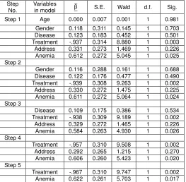
Table 9: The results of (Backward method) for select
sig.variables
Step No.
Variables
in model βu S.E. Wald d.f. Sig. Step 1 Age 0.000 0.007 0.001 1 0.981
Gender 0.118 0.311 0.145 1 0.703 Disease 0.123 0.183 0.452 1 0.501 Treatment -.937 0.314 8.880 1 0.003 Address 0.331 0.273 1.469 1 0.226 Anemia 0.612 0.272 5.045 1 0.025 Step 2
Gender 0.116 0.288 0.161 1 0.688 Disease 0.122 0.176 0.477 1 0.490 Treatment -.939 0.308 9.263 1 0.002 Address 0.330 0.272 1.475 1 0.225 Anemia 0.611 0.272 5.064 1 0.024 Step 3
Disease 0.109 0.175 0.386 1 0.534 Treatment -.938 0.309 9.189 1 0.002 Address 0.329 0.272 1.465 1 0.226 Anemia 0.584 0.263 4.930 1 0.026 Step 4
Treatment -.957 0.310 9.508 1 0.002 Address 0.292 0.265 1.215 1 0.270 Anemia 0.606 0.260 5.423 1 0.020 Step 5
Treatment -.967 0.310 9.747 1 0.002 Anemia 0.622 0.261 5.703 1 0.017
Therefore we get only two significant variables with Cox model as follows:
Y λt) exp (−0.967f+ 0.622) and
Y = Ln λ(/W(,W{,W,W,W,W) λ() =
−0.967f+ 0.622
Table 10:Select the best model of likelihood ratio statistic as follows:
Step No.
-2log Likelihood (present) model
-2log Liklihood (reference) model
LR
.Chi-square d.f Sig. Step 1 407.446 390.595 16.851 6 0.011 Step 2 407.446 390.595 16.850 5 0.005 Step 3 407.446 390.759 16.687 4 0.002 Step 4 407.446 391.134 16.312 3 0.001 Step 5 407.446 392.372 15.074 2 0.001
Table (10) showing that model in step (5) is more significant than others. Also, the probability of survival for patients is always decreasing as showing as in (Fig. 2).
Figure 2: Cumulative survival function for patients.
11. Conclusion
1- We find from data analysis that most ratio of death (%54.54) in the first month of censored (September) and most death that patients of age under (20 years) is (%42.46).
2- Most death is the patients of female (% 63) and most common disease is (Acute myeloid leukemia) with ratio (%43.8) and has most ratio of death (% 63.63).
3- From the results of Cox- reg. model we have only two sig. variables (Treatment and Anemia).
4- Most risk at survival time at (0- 20) days with probability survival (0.0039) and we find that the risk of death is increasing with time, that is mean the disease still continuo.
12. References
[1] Agresti A.”Categorical Data Analysis”. John Wiley and Sons, New York, 1990.
[2] Bender, ”Generating survival times to simulate cox Proportional hazard models”, sander for schung sbereich,386, p338, 2003.
[3] Cox D.R., ”partial likelihood”, biometric , 62, 2 , p(269-276), 1975.
[4] Inger person ,” Essays on the Assumption of Proportional Hazards in Cox Regression” Uppsala University. Sweden, 2002
[5] Izenman , A.J. and Tran, L.T.,”Estimation of the survival function and hazard rate”, Journal of stat planning and Inference, V .24,p(233-247), 1990.
INTERNATIONAL JOURNAL OF SCIENTIFIC & TECHNOLOGY RESEARCH VOLUME 3, ISSUE 11, NOVEMBER 2014 ISSN 2277-8616
320
[7] Nihal Ata and M.Tekin Säozer, ” cox regression model with Nonprortional hazard applied to lung cancer survival”, Hacettepe Journal of Mathematics and Statistics,vol.36, No.2 , p(157-167), 2007.