Article
Affecting Wingtip Vortex Using Wing Surface
Contours
Sidaard Gunasekaran1,†,‡, Nathan Thomas1,‡
1 2 3 4 5 6 7 8 9 10 11 12 13
1 AssistantProfessor,UniversityofDayton;[email protected]
2 UndergraduateStudent,UniversityofDayton;[email protected]
* Correspondence:[email protected];Tel.:+1-937-229-5345
Abstract: The aerodynamic efficiency of a NACA 0012 AR 4 wing was affected through periodiccontoursalignedintheflowdirection resemblinga “wrinkled”texture. Streamwiseand cross-stream Particle Image Velocimetry (PIV) wereconducted at theUniversity of Dayton Low SpeedWindTunnel(UD-LSWT)aroundReynoldsnumberof135,000ontheNACA0012AR4wing withandwithoutsurfacecontours.Wingswith6contoursectionswasdesignedbysplinefittingtwo NACA0012airfoilprofilesinthespanwisedirection. Both2D(wall-to-wallmodel)configuration and3Dconfigurationofthewingsweretestedtodeterminetheeffectsofsurfacecontoursonthe parasiteandinduceddragofthewing.StreamwisePIVresultsindicatedanincreaseinmomentum deficitinthewakeofthemid-contourregionduetoenhancedboundarylayerseparationfromthe uppersurfaceofthemid-contourregion. Thecross-streamPIVresultsindicatedadecreaseinthe magnitude of azimuthal velocity, circulation and RMS quantities in the wingtipvortex with the surface contours. Thereductioninthewingtipvortexpropertiesindicatesthatthecontourswere effectiveinblockingthespanwiseflowfeedingintothewingtipvortexonthesurfaceofthewing.
Keywords:AerodynamicEfficiency;Wrinkled/ContouredSurface;SurfaceFlow 14
1. Introduction 15
A major inconvenience in the aerospace industry today is the fact that most conventional aircraft 16
cannot operate under optimal conditions (maximum Lift-to-Drag ratio) because it is too slow. Two 17
major components of drag which affects the aerodynamic efficiency are the parasitic and induced 18
drag. The lift-induced drag is responsible for more than 70% of the total drag of the aircraft during 19
take-off and landing and about 5-15% of the total drag during cruising [1]. By far, no universal 20
mathematical relation exists which relates the physics and properties of the wingtip vortex rollup 21
process, its evolution and the induced drag. Over the years, numerous methods to reduce induced 22
drag have been conceived and implemented. Methods such as installing end plates at wingtips, 23
winglets (most common), lift distribution tailoring (By changing the deflection of flaps on the wing), 24
active/passive flow control methods (Blowing or Suction of air at the wingtip), etc. have been 25
employed over the years to affect the aerodynamic efficiency of the wing. But out of all the methods 26
mentioned above, the total reduction in drag so far has only been 5-7%. The non-satisfactory 27
performance of these methods is due to the ineffective influence of the wingtip vortex roll-up 28
process. A recent study performed by Gunasekaran and Altman [2] has shown that there might be an 29
interesting interaction between the parasite drag of the wing and induced drag of the wing caused by 30
wingtip vortices. By manipulating the spanwise flow over the wing, it is hypothesized that the rollup 31
process of wingtip vortex will be affected which changes the induced drag contribution to total drag. 32
The research documented in this paper tests this hypothesis by contouring the surface of the wing to 33
affect the spanwise flow. 34
Wings with unintentional contouring can be found in airplanes such as light-weight sport (Ex: 35
CGS Hawk - gross weight around 500 lbs.) which consists of multiple ribs covered by a Dacron 36
fabric. As a result, the surface of the wings is inherently bumpy as the Dacron fabric lags between 37
two ribs due to its own weight. In this region, the airfoil profile of the wing deviates from the intended 38
airfoil profile. As a result, most of the wing surface doesn’t have the intended airfoil profile! But, it is 39
advertised that even without a smooth surface of the wing, the CGS Hawk light weight sport airplane 40
delivers good performance [3]. 41
Figure 1.Front and Top View of CGS Hawk light-weight sport aircraft. It is hypothesized that the ribs act as ridges which disrupt the spanwise flow over the wings thereby increasing the efficiency.
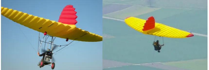
Surface contours similar to the ones observed on the CGS Hawk (Figure 1) can also be seen on 42
inflatable wings. One such aircraft with inflatable wings is the Woopy-Fly [4] shown in Figure 2. 43
Ridges can be seen all over the wing surface which might affect surface flow around the wing. It is 44
hypothesized that such ridges or bumps affects the balance of lift induced and parasite drag of the 45
wing. 46
Figure 2. Woopy-Fly aircraft with inflatable wing. Similar to CGS Hawk, the inflatable wing has chordwise bumps and ridges which is hypothesized to affect the surface flow direction.
Numerous studies have been conducted concerning on the study of inflatable wings. The natural 47
contoured shape due to inflation pockets resembles spanwise contours although unintentional. As 48
such some very interesting, and useful data on the resultant aerodynamic efficiency of a wing without 49
a smooth surface is available for review. A study conducted by Zhang et al [5] found a number of 50
differences in the aerodynamic efficiency when chord-wise contours were introduced to an Eppeler 51
were performed at low angles of attack and at multiple Reynolds numbers on a 2D wall-to-wall 53
model and a 3D model of Eppeler 398 and NACA 4318 wings with and without surface contours. 54
Interestingly enough, it was found that the inflatable wing noticeably reduced separation of the flow 55
when compared to its smooth counterpart for the Reynolds number of 25000 and at an angle of attack 56
of 4 as shown in Figure 3. However, this reduction was found to not necessarily indicate improved 57
flight performance. The results from [5] indicates that for certain Reynolds numbers and high angles 58
of attack, the inflatable wing had a noticeably higher aerodynamic efficiency. However, at lower 59
angles of attack, the smooth wings were found to perform better. 60
Figure 3.Flow visualization of Eppler 398 a.) bumpy b.) smooth wing at Re = 25000, = 4 degrees [5]
The ridges and bumps essentially increases the roughness of the surface of the wing and it has 61
been shown through experimental investigations that the a “rough” airfoil surface will perform better 62
than a “smooth” airfoil section at lower Reynolds numbers (40-50,000) [6]. Even at high Reynolds 63
numbers “riblets” were used to reduce frictional drag [7]. Previous experimental measurements and 64
numerical calculations have shown a possibility of achieving up to 10% drag reduction in the total 65
frictional drag on an immersed and textured surface [8]. Most of the concepts to increase surface 66
roughness was inspired from biological observations such as denticles on sharks. This raised the 67
possibility of achieving drag reduction using streamwise grooves [9], [10],[11],[12] as shown in Figure 68
4b [13]. These streamwise grooves or riblets are proven to be effective is reducing cross-stream 69
velocity fluctuations. The low velocity fluid flow in the valleys of the riblets produces very low-shear 70
stresses across most of the surface of the riblets. Also, the cross-stream velocity fluctuations inside 71
the riblet valleys were found to be much lower than the cross-stream velocity fluctuations above a flat 72
plate [13]. The reduced cross-stream velocity fluctuations along with reduced wall shear stress results 73
in a lower skin friction drag with riblets. 74
Similar to the riblets, a surface with sinusoidal wavy pattern was studied in [14] where the groves 75
are oriented along the streamwise direction. This type of surface is also known as “wrinkled” texture. 76
The research presented in this paper has a similar textured surface on the upper and lower surface of 77
the wing. The wrinkled surface also was found to reduce the cross-stream fluctuations and reduces 78
shear stress similar to riblets shown in Figure 4. The riblets with an aspect ratio close to unity gave the 79
highest reduction in total drag [14]. The reduced cross-stream fluctuations by the riblets are highly 80
desired in a finite wing which has an added induced drag component. With the rollup of wingtip 81
vortices, creates a spanwise/cross-stream component of flow on the upper and lower surface of the 82
wing. The spanwise flow feeds into the rollup of the wingtip vortices increasing the vortex strength. 83
The riblets could act as a boundary layer fence preventing the spanwise flow that feeds into the 84
wingtip vortex. Therefore, it is hypothesized that the properties in the wingtip vortex will be affected 85
due to the presence of the spanwise riblets. 86
2. Experimental Setup 87
2.1. Test Model 88
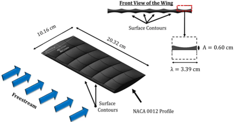
A NACA 0012 AR 2 semispan wing was designed in SolidWorks with surface contours along 89
the span of the wing as shown in Figure 5. The surface contours are created by a series of segments 90
along the span of the wing. Each contoured segment is designed by having a NACA 0012 airfoil 91
profile at the boundaries and spline fitting in-between. A total of 6 contour segments were modeled 92
and sensitivity analysis was done on the aerodynamic forces as a function of the length and number 93
of contoured areas. conventional NACA 0012 AR 4 wing without any surface contours was also 94
modeled and printed. 95
Figure 5.SolidWorks model of an AR 4 NACA 0012 wing with 12 surface contoured segments. The wing area in between each contour do not have NACA 0012 profile.
The surface area of the wing with the contours was 896.7 and the surface area of the wing 96
without the contours was 864.5 which is a 3% increase in surface area. The presence of contours 97
create a variable airfoil profile between any two of the NACA 0012 profile sections. The wavelength 98
of each contour is 3.39cm and the amplitude A of each contour is 0.60 cm. There is a 53% reduction 99
midpoint section as the leading-edge mimics a cylindrical shape. The schematic of the profile sections 101
in-between each contour segment is shown in Figure 6. 102
Figure 6.Profile transformation as an effect of wing contours. Profiles are plotted symmetrically on the Y-axis vs. the characteristic length.
2.2. Wind Tunnel 103
All the experiments were conducted at the University of Dayton Low Speed Wind Tunnel 104
(UD-LSWT). The UD-LSWT has a 16:1 contraction ratio, 6 anti-turbulence screens and 4 105
interchangeable 76.2cm x 76.2cm x 243.8cm (30” x 30” x 96”) test sections. The test section is 106
convertible from a closed jet configuration to an open jet configuration with the freestream range 107
of 6.7m/s (20 ft/s) to 40m/s (140 ft/s) at a freestream turbulence intensity below 0.1% measured by 108
hot-wire anemometer. The tunnel also has the ability to vary the freestream velocity profile at up to 109
5 Hz and over 50% velocity amplitude using a downstream shuttering system. All the experiments 110
mentioned in the paper were done in the open jet configuration where an inlet of 76.2 cm x 76.2 cm 111
opens to a pressure sealed plenum. The effective length of the test section in the open jet configuration 112
is 182cm (72”). A 137cm x 137cm (44” x 44”) collector collects the expanded air on its return to the 113
diffuser. A photo of the UD-LSWT open jet configuration is shown in Figure 7. The velocity variation 114
for a given RPM of the wind tunnel fan is found using a Pitot tube connected to an Omega differential 115
pressure transducer (Range: 0 – 6.9 kPa). 116
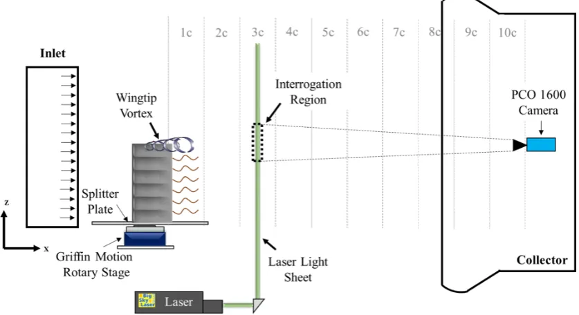
2.3. PIV Experiments 117
Streamwise Particle Image Velocimetry (PIV) and cross-stream PIV were conducted in the free 118
shear layer and the wingtip vortex of the semispan wing models with and without the holes. The 119
PIV measurements were obtained using a Vicount smoke seeder with glycerin oil and a 200 mJ/pulse 120
Nd: YAG frequency doubled laser (Quantel Twins CFR 300). A Cooke Corporation PCO 1600 camera 121
(1600 x 1200 pixel array) with a 105 mm Nikon lens was used to capture the images. One plano-convex 122
lens and one plano-concave lens were used in series to convert the laser beam into a sheet. The 123
laser and the camera were triggered simultaneously by a Quantum composer pulse generator. In 124
each test case, over 700 image pairs were obtained and processed using ISSI Digital Particle Image 125
Velocimetry (DPIV) software. A total of 2 iterations were performed during PIV processing with 126
64-pixel interrogation windows in the first iteration and 32-pixel interrogation windows in the second 127
iteration. Both the streamwise and cross-stream PIV interrogations were conducted a Reynolds 128
number of 135,000. The test matrix for the PIV experiment is shown in Table 1. 129
Table 1.Test Matrix for Free Shear Layer (FSL) and wingtip vortex interrogation using PIV
PIV Cases Wing Model Angle of Attack (Degrees) Interrogation Location
Streamwise FSL Baseline and Wrinkled 0, 2, 4, 6, 8 Behind TE
Cross-stream WV Baseline and Wrinkled 2, 4, 6, 8 3 Chord Lengths Downstream
2.4. Streamwise PIV Setup 130
The streamwise PIV was done in the FSL of the contoured wing with splitter plate on both 131
wingtips to prevent wingtip vortex formation. The interrogation window was placed near the trailing 132
edge of the wing as shown in Figure 8a. Two PIV interrogation regions were considered: one behind 133
the NACA-0012 section and one behind the middle of the contour section. A Nikon 105 mm lens was 134
used in the streamwise PIV case which gave a spatial resolution of 292 pix/cm in both axes. The size 135
of the field of view was 5.5 cm x 4.1 cm which gave a magnification factor of 0.21 (Figure 8b). The 136
for the images were set to obtain an average particle displacement of 8-10 pixels in the wake of the 137
wing. The wing model was moved in the spanwise direction to perform PIV behind the mid-contour 138
to maintain the same magnification factor and resolution. 139
2.5. Cross-stream PIV Setup 140
The cross-stream PIV was done to determine the effects of spanwise contours on the roll-up of 141
the wingtip vortex. The wingtip vortex from the baseline NACA 0012 and the contoured wing was 142
interrogated at multiple angles of attack at a Reynolds number of 135,000 as mentioned in Table 1. 143
The schematic of the cross-stream PIV setup is shown in Figure 9. The cross-stream interrogation 144
window is 3 chord lengths downstream from the trailing edge of the wing. The PCO 1600 camera 145
was located at more than 10 chord lengths downstream from the trailing edge of the wing, inside the 146
collector and the effect of the camera being in the flow will comparatively be less. Due to the long 147
object distance, a Nikon 200 mm with extension rings were used to focus the interrogation region. The 148
spatial resolution of the field of view was 350 pix/cm, and the size of the field of view was around 4.6 149
cm x 3.4 cm which gave a magnification factor of 0.25. The time delay between the laser pulses was 150
changed at each angle of attack to obtain 8-10 particle displacement at the boundary of the wingtip 151
vortex. 152
Figure 9.Schematic of cross-stream PIV setup for wingtip vortex interrogation.
3. Results 153
3.1. Streamwise PIV Results 154
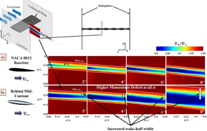
The streamwise velocity Ux was determined behind the NACA-0012 wall-to-wall model (Figure 155
10a) and the mid-contour section (Figure 10b). It is evident from the contours that the momentum 156
deficit behind the mid-contour profile is greater than the baseline. There is also an apparent increase 157
in the wake half width ( - identified by the location of 99%U∞) behind the mid-contour profiles when 158
compared to the baseline. The wake half-width of the two cases are similar until angle of attack. The 159
differences in the wake-half width between the two cases increases significantly at 6 and 8 angle of 160
attack. Apart from the wake-half width, the magnitude of the Ux in the wake is comparatively lower 161
in the mid-contour at all angles of attack. The momentum deficit profiles shown in Figure 10 helps 162
to emphasize the difference in wake momentum deficit. The profiles were obtained by averaging 163
10 columns of data from the center of the field of view. The streamwise velocity is normalized by 164
the freestream and plotted against the normalized wake-half width (y/L0). The momentum deficit 165
behind the mid-contour contour is greater than all the NACA 0012 baseline angle of attack cases. 166
deficit of the baseline at 8 case. The increased momentum deficit for a thin mid-contour profile might 168
be due to the separation of the boundary layer from the upper surface of the wing. 169
Figure 10.Normalized streamwise contours in the FSL wake of a.) Baseline NACA 0012 wall-to-wall model and b) Behind mid-contour of the contoured wing wall-to-wall model. The momentum deficit and the wake half-width behind mid-contour is greater at all angles of attack when compared to the baseline.
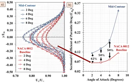
The momentum deficit profiles shown in Figure 11a was used to determine the sectional drag 170
coefficient of the NACA 0012 baseline profile and the mid-contour profile. The sectional drag 171
coefficient was found by integrating the momentum deficit profiles according to the equation, 172
CD= ρU
2 ∞ q∞S
Z U
x
U∞(1− Ux
U∞)dy (1)
where is the density of the fluid, is the freestream velocity, is the reference area of the wing, 173
and is the dynamic pressure the experiment was conducted at. Equation 1 was obtained from the 174
momentum equation assuming steady, inviscid and incompressible flow with no body force and no 175
streamwise pressure gradient. The sectional drag coefficient for both cases increases non-linearly 176
with angle of attack. But the magnitude of the drag coefficient behind the mid-contour profile is 177
significantly larger than the baseline NACA 0012 profile. Even though the normalized momentum 178
deficit profiles in Figure 11a shows similar trend in both cases, the wake-half width is significantly 179
larger in the mid-contour case as seen in Figure 10b. At 8 angle of attack, the streamwise velocity 180
contours shows a significant increase in wake-half width when compared to all the other angles 181
of attack. Therefore, the drag coefficient of the mid-contour profile at 8 also shows a significantly 182
higher magnitude when compared to the baseline. It is very likely that the drag coefficient of the 183
sections in-between the mid-contour and the NACA 0012 profile lies within the differences in the 184
drag coefficient magnitude seen in Figure 11b between the two cases. In order to determine the effect 185
of increased momentum deficit in the wingtip vortex, the cross-stream PIV results are analyzed in the 186
Figure 11. a) Momentum deficit profiles taken from contours shown in Figure 10 for the baseline and the mid-contour case at different angle of attack. The profiles indicate a significant increase in the momentum deficit at all angles of attack when compare to the baseline. b) Sectional parasitic drag coefficient variation with angle of attack for the two cases. The Cd is much greater behind the mid-contour profile when compared to the baseline at all angles of attack.
3.2. Wingtip Vortex Results 188
The intention behind the contoured wing is to determine the effect of the contours on the wingtip 189
vortex properties. The contours acting like a riblet were hypothesized to block the spanwise flow over 190
the wing thereby reducing the strength of the wingtip vortex. The properties of the wingtip vortex are 191
discussed in this section starting with the wingtip vortex wandering. It is important to quantify the 192
vortex wandering since increased level of vortex wandering biases the mean velocity component to 193
be lower than the actual value. It also makes the appearance of a larger vortex. The vortex wandering 194
was quantified by tracking the center of the vortex across all individual image pairs. The center of the 195
vortex was identified through scaled Q-criterion. The Q-criterion is a well-known method to identify 196
vortices in a flowfield. The equation for Q-criterion is, 197
Q= 1 2(||Ω||
2− ||R||2) (2)
where||Ω||is the absolute magnitude of vorticity given by 198
Ω= 1
2
∂Uz
∂y −
∂Uy ∂z
(3)
and||R||is the absolute magnitude of strain rate given by 199
R= 1 2
∂Uz
∂y +
∂Uy ∂z
The scaled Q-criterion (Qs) is the shear strain normalized Q-criterion,
Qs = 1 2
||Ω||2
||R||2 −1
(5)
An example plot of the normalized Q-criterion of the contoured wing case at 4 angle of attack is 200
shown in Figure 12. The maximum Q-criterion was identified as the center of the wingtip vortex at 201
each instantaneous image pairs. The vortex centers identified through this method is shown in Figure 202
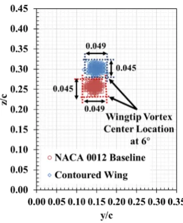
13 for 6 angle of attack for both the baseline NACA 0012 and the contoured wing. 203
Figure 12. Using scaled Q-criterion to determine the vortex center at each individual image pairs to quantify vortex wandering.
Figure 13 clearly shows the variation of the vortex center location for all 700 image pairs captured 204
for both cases at 6 angle of attack. The wandering of the vortex center for both cases was contained 205
within the 5% chord which is less than 5 mm. Therefore, significant deviations of the vortex center 206
are not observed. The vortex wandering was corrected by centering all the vortex center at a single 207
location. The resultant deviations in the peak Uz and Uy azimuthal velocities were less than 5%. 208
Whereas higher percentage differences between the baseline and the contoured wing were seen in 209
the azimuthal velocity contours shown in Figure 14. 210
Figure 14. Variation of azimuthal velocity for a.) baseline NACA 0012 wing b.) contoured wing for different angles of attack. The magnitude of the azimuthal velocity of the contoured wing is lower than the baseline for all angle of attack.
The magnitude of the peak azimuthal velocity increases with increase in angle of attack for both 211
cases as expected. The positive contour of the Uz velocity indicates the wingtip vortex rolling up 212
from the free shear layer into the wingtip vortex (can be seen clearly in vorticity plot (Figure 16)). The 213
magnitudes of the azimuthal velocities in the contoured wing case are lower than the baseline case 214
at all angles of attack indicating that the cross-stream momentum of the wingtip vortex is reduced 215
by the presence of the contours. This decrement in the azimuthal velocity could be due to contours 216
inhibiting the spanwise flow that feeds into the wingtip vortex. The differences in the azimuthal 217
velocity can be clearly seen by obtaining profiles from the contours as shown in Figure 15a. The 218
normalized azimuthal velocity profiles in Figure 15a are taken horizontally parallel to the wingspan 219
and hence the free shear layer. The azimuthal velocity profiles are plotted against the wingtip vortex 220
radius normalized by the radius of the vortex boundary. The vortex boundary is identified as the 221
location at which the maximum azimuthal velocity occurs. The contoured wing profiles clearly 222
show a decrement in the azimuthal velocity profile when compared to the baseline at all angles of 223
attack. The differences between the baseline and the contoured wing cases in the azimuthal velocity 224
are preserved on the positive and negative side of the profile indicating that the vortex is nearly 225
symmetric and the influence of the free shear layer on the wingtip vortex is minimal. The azimuthal 226
velocity of the contoured wing at 8 angle of attack has the same magnitude as the 6 angle of attack of 227
the baseline case. The peak azimuthal velocity is also plotted against the angle of attack for both the 228
cases in Figure 15b. A nearly linear variation in the azimuthal velocity profiles can be seen in both the 229
cases as shown by the linear regression equation. The differences in the peak azimuthal velocity is 230
a 43% reduction in the magnitude of the peak azimuthal velocity when compared to the baseline and 232
at , only 6% reduction is observed. The reduction could be due to the ineffectiveness of the ridges at 233
higher angles of attack preventing the spanwise flow. 234
Figure 15. a) Normalized Azimuthal velocity profiles of baseline and contoured wing for varying angles of attack. b) Peak azimuthal velocity measured on horizontal line passing through vortex centers.
According to Batchelor’s model (Batchelor (1964) (), any change in the peak azimuthal velocity 235
will result a change in the radius of the wingtip vortex provided that the circulation remains the same. 236
To quantify the changes in the circulation between the two cases, x-vorticity of the wingtip vortex was 237
calculated using Equation 3. The velocity gradients in Equation 3 was determined using the central 238
difference technique. The normalized x-vorticity contours for the baseline and the contoured wing is 239
shown in Figure 16. 240
The vorticity magnitude is higher at the wingtip vortex core as expected and increases with angle 241
of attack for both the cases. However, the contoured wing case show a lower vorticity magnitude on 242
comparison with the baseline across all angles of attack. This effectively indicates that the contours 243
on the surface of the wing effectively altered the rollup process of the wingtip vortex. The normalized 244
x-vorticity values of 0.15, 0.20 and 0.30 are highlighted in white to indicate the presence of the free 245
shear layer (FSL) in all angles of attack for both cases. A clear distinction between the wingtip vortex 246
and the free shear layer which rolls up into the vortex can be seen. It was postulated in Gunasekaran 247
and Altman [2] that the free shear layer interacts with the wingtip vortex rollup process at lower 248
angles of attack and moves away from the wingtip vortex as the downwash increases at higher angles 249
of attack. Figure 16 indicates similar behavior where the distance between the wingtip vortex core and 250
the free shear layer increases with increase in angle of attack for both the baseline and the contoured 251
wing cases. 252
To quantify the reduction in the wingtip vortex strength, wingtip vortex circulation was 253
determined by integrating the vorticity as shown in Equation 6. 254
Γ=
Z Z
ω.ds (6)
whereΓis the circulation,ωis the vorticity anddsis the incremental surface area. After determining 255
the wingtip vortex center through Q-criterion, several concentric circles were made around the vortex 256
center to determine the circulation as a function of wingtip vortex radius. An example of a circulation 257
plot obtained through this procedure is shown in Figure 17. 258
Figure 17.Variation of circulation as a function of vortex radius. The circulation was determined by taking concentric circles from the vortex center.
Once the circulation variation is obtained, the profile is fitted to an ideal Lamb-Oseen vortex 259
model described by Equation 7 to determine the total circulationΓ0and vortex core radiusrc. 260
Γ(r) =Γ0
1−exp
−r2
r2
c
This method of finding circulation was developed by Stevens (2013) and has been employed in 261
Corkery and Babinsky (2017) and Stevens and Babinsky (2017) to determine circulation of vortices 262
emanating from pitching and plunging wings. The Lamb-Oseen model is fitted with the experimental 263
data for the baseline NACA 0012 wing at 8 degree angle of attack by changing the total circulation 264
value (Γ0) (Figure 18). A value of 0.3m2/sgave the highestR2value of 0.98. Similar fit was obtained 265
for all angles of attack by changingΓ0the that gives a higherR2value for both the baseline and the 266
contoured wing case. The averageR2value for all the cases was 0.98. 267
Figure 18. Determining total circulation of the wingtip vortex by fitting the experimental data with
the Lamb-Oseen vortex model. The current graph is for the baseline NACA 0012 wing at 8◦angle of
attack.
The normalized circulation obtained by this method for all angles of attack is shown in Figure 268
19 for the NACA 0012 baseline wing and the contoured wing. The circulation increases linearly (as 269
denoted by theR2values) as a function of angle of attack for both cases. This is expected as the 270
variation of the lift coefficient with angle of attack is also linear for both cases at the range of angle 271
of attack shown. The magnitude of the circulation however is different between the both cases. The 272
contoured wing case circulation magnitude is lower than the baseline wing across all angles of attack. 273
The differences in the circulation however decreases with increase in angle of attack from 34% at 2◦to 274
6% at 8◦angle of attack. Similar trend is seen in the peak azimuthal velocity as a function of angle of 275
attack (Figure 15b). The average reduction in circulation across angles of attack however is around 276
20% between the baseline and the contoured wing. This result once again indicates that the ridges on 277
Figure 19.Peak circulation as a function of angle of attack.
Figure 16 showed disturbances in the vorticity of the free shear layer in the contoured case. This 279
could occur due to the increased turbulence level in the free shear layer caused by the presence of the 280
surface contour. To quantify the effect of fluctuating quantities in the wingtip vortex, the normalized 281
UZ RMSwas determined for both the baseline and the contoured wing case. TheUZ RMSrepresents the 282
fluctuations in velocity about the Z-axis which is perpendicular to the span of the wing. TheUZ RMS 283
is calculated by, 284
UZ RMS= q
(u0
z)2 (8)
where u0z is the fluctuating velocity about the Z-axis. In the baseline case, higher UZ RMS is 285
concentrated in the wingtip vortex core when compared to theUZ RMS in the free shear layer and 286
in the boundary of the vortex (Figure 20). In the contoured wing case however, the magnitude of 287
UZ RMSis distributed throughout the vortex. However, the concentration of theUZ RMSin the vortex 288
center is comparatively reduced in the contoured wing case. The normalizedUZ RMS values of and 289
are highlighted in white to distinctly observe the wingtip vortex and the FSL. A distinct separation 290
is seen between the wingtip vortex and the FSL in both the cases at the wingtip vortex-FSL interface 291
in Figure 20. TheUZ RMSat this interface is lower than the wingtip vortex and the FSL which could 292
potentially indicate the separation from the wingtip vortex and the free shear layer. TheUZ RMSin 293
the free shear layer is increased in the contoured wing when compared to the baseline wing due to 294
Figure 20.The ZRMS plot shows the contoured wing having a lower ZRMS in its core. However, the increased FSL vortex-core interaction may be clearly noted for the contoured wing case. At 4 there is lower ZRMS measured at the FSL-vortex interface which may indicate separation between the FSL and the wingtip vortex.
4. Conclusions 296
A NACA 0012 semi-span wing with contours resembling “wrinkled” texture was investigated 297
to determine the changes in the free shear layer and the wingtip vortex. The semi-span wing features 298
6 contours which were hypothesized to reduce the spanwise flow component over the wing which 299
feeds into the wingtip vortex. The important results are as follows: 300
• Larger momentum deficit along with larger wake half width was observed in the free shear layer 301
in the wake of the mid-contour section when compared to the baseline. The average increase in 302
the momentum deficit was around 8% excluding the 8 angle of attack. The momentum deficit was 303
significantly greater at 8 angle of attack due to boundary layer separation. This is a consequence 304
of a higher sectional drag coefficient caused by separation effects at lower angles of attack for the 305
mid-contour profile shape. The increased drag coefficient in the contoured wing is due to the 306
presence of a round leading edge causing separation at lower angle of attack. 307
• Even though the momentum deficit increased in the free shear layer in the contoured wing case, 308
the peak azimuthal velocity of the wingtip vortex was measurably lower than the baseline (43% 309
at 2 ranging up to 6% at 8) at all angles of attack. 310
• The peak vorticity at the wingtip vortex core decreased from 47% at 2 to 5% at 8 angle of attack 311
in the contoured wing case when compared to the baseline. This indicates that the rollup of the 312
wingtip vortex was affected by the presence of the contours. 313
• The overall circulation of the wingtip vortex also reduced in the contoured wing case by an 314
average of 20% across all angles of attack when compared to the baseline. 315
• The contoured wing case shows increased ZRMS in the FSL feeding into the wingtip vortex. 316
However, the core of the contoured wing vortex has a lower ZRMS value when compared to 317
Conflicts of Interest:The authors declare no conflict of interest. 319
Abbreviations 320
The following abbreviations are used in this manuscript: 321
322
α- Angle of Attack (Degrees) 323
AR - Aspect Ratio 324
c- Chord Length (m) 325
Γ(r)- Circulation as a function of vortex radius (m2/s) 326
CD- Coefficient of Drag 327
CD0- Coefficient of Sectional Drag 328
q∞- Dynamic pressure (N/m2) 329
u0y- Fluctuating Velocity in Y-axis (m/s) 330
u0z- Fluctuating Velocity in Z-axis (m/s) 331
U∞- Freestream velocity (m/s) 332
η- Non-dimensional vortex radius 333
σy- RMS wandering amplitude component in y-axis (m) 334
σz- RMS wandering amplitude component in z-axis (m) 335
R- Strain rate (1/s) 336
t- Thickness of airfoil (m) 337
Γ0- Total Circulation (m2/s) 338
UZ RMS-UZvelocity component RMS 339
UY RMS-UYvelocity component RMS 340
UX- Velocity in X-direction (m/s) 341
UY- Velocity in Y-direction (m/s) 342
UZ- Velocity in Z-direction (m/s) 343
Ω- Vorticity (1/s) 344
r- Vortex radius (m) 345
rc- Vortex core radius (m) 346
b- Wingspan (m) 347
S- Wing reference area (m2) 348
349
References 350
1. Butler, S.F.J., "Aircraft Drag Prediction for Project Appraisal and Performance Estimation," AGARD-CP-124,
351
1973, pp. 6-1 - 6-50 352
2. Gunasekaran, Sidaard, Altman, Aaron, “Is There a Relationship Between the Free Shear Layer and
353
the Wingtip Vortex”, 54th AIAA Aerospace Science Symposium (SCITECH), January, 2016, San Diego, 354
California. https://doi.org/10.2514/6.2016-1068 355
3. CGS Aviation, 440 Airport Road Lake Wales, FL. United States. CGS Hawk - http://www.cgsaviation.com/
356
4. Woopy Company.Woopy Fly Inflatable Wing Aircraft. - http://fly.woopyjump.com/
357
5. Feng Zhang, Kevan J. Ghobadi, Grant Spencer, Justin Krofta, Raymond P. LeBeau, Jr.5, Mark
358
McQuilling, “Examination of Three-Dimensional Flow over a Chambered Inflatable Wing”, 52nd 359
AIAA Aerospace Science Symposium (SCITECH), January 2014, National Harbor, Maryland.
360
https://doi.org/10.2514/6.2014-0556 361
6. J.H. McMasters and M.L. Henderson. “Low-speed single element airfoil synthesis.” Technical Soaring,
362
6:1–21, 1980. 363
7. Walsh, M. J. and Weinstein, L., “Drag and heat-transfer characteristics of small longitudinally ribbed
364
8. Viswanath, P. R., “Aircraft viscous drag reduction using riblets,” Prog. Aerospace. Sci. 38, 571–600 (2002) 366
https://doi.org/10.1016/S0376-0421(02)00048-9 367
9. Bechert, D., Hoppe, G., and Reif, W.-E., “On the drag reduction of the shark skin,” AIAA Paper No. 85-0546,
368
1985.4. [ 369
10. Bechert, D. W., Bruse, M., and Hage, W., “Experiments with three-dimensional riblets as an Idealized model
370
of shark skin,” Exp. Fluids 28, 403–412 (2000). https://doi.org/10.1007/s003480050400 371
11. Walsh, M. J., “Riblets,” in Viscous Drag Reduction in Boundary Layers, edited by D. M. Bushnell (AIAA,
372
1990), Vol. 1, pp. 203–261. 373
12. Lee S.-J., Lee S.-H. (2001) Flow field analysis of a turbulent boundary layer over a riblet surface. Exp. Fluids
374
30:153–166https://doi.org/10.1007/s003480000150 375
13. Raayai-Ardakani, Shabnam, and Gareth H. McKinley. "Drag reduction using wrinkled surfaces in
376
high Reynolds number laminar boundary layer flows." Physics of Fluids 29, no. 9 (2017): 093605.
377
https://doi.org/10.1063/1.4995566 378
14. G. K. Batchelor (1964). “Axial flow in trailing line vortices”. Journal of Fluid Mechanics, 20, pp 645-658
379
![Figure 3. Flow visualization of Eppler 398 a.) bumpy b.) smooth wing at Re = 25000, = 4 degrees [5]](https://thumb-us.123doks.com/thumbv2/123dok_us/1078381.1608574/3.595.156.439.582.728/figure-flow-visualization-eppler-bumpy-smooth-wing-degrees.webp)