Unsupervised Metric Learning using low dimensional
embedding
Parag Jain
[email protected]
Indian Institute of Technology, Hyderabad
Unsupervised metric learning has been generally studied as a byproduct of dimensionality reduction or manifold learning techniques. Manifold learning techniques like Diffusion maps, Laplacian eigenmaps has a special property that embedded space is Euclidean. Although laplacian eigenmaps can provide us with some (dis)similarity information it does not provide with a metric which can further be used on out-of-sample data. On other hand supervised metric learning technique like ITML which can learn a metric needs labeled data for learning. In this work propose methods for incremental unsupervised metric learning. In first approach Laplacian eigenmaps is used along with Information Theoretic Metric Learning(ITML) to form an unsupervised metric learning method. We first project data into a low dimensional manifold using Laplacian eigenmaps, in embedded space we use euclidean distance to get an idea of similarity between points. If euclidean distance between points in embedded space is below a threshold t1 value we consider them as similar points and if it is greater than a
certain threshold t2 we consider them as dissimilar points. Using this we collect a batch of
similar and dissimilar points which are then used as a constraints for ITML algorithm and learn a metric. To prove this concept we have tested our approach on various UCI machine learning datasets. In second approach we propose Incremental Diffusion Maps by updating SVD in a batch-wise manner.
Keywords: unsupervised, metric learning, embedding learning, laplacian, information theoretic, diffusion maps
1
Unsupervised Information Theoretic Metric
Learn-ing usLearn-ing Laplacian eigenmaps
1.1
Laplacian eigenmaps
Laplacian eigenmaps learns a low dimensional representation of the data such that the local geometry is optimally preserved, this low-dimensional manifold approximate the geometric structure of data. Steps below describes the methods in detail.
Consider set of data points X ∈ RN, goal of laplacian eigenmaps is to find an embedding in
m dimensional space where m < N preserving the local properties of data.
July 2015
1. Construct a graph G(V, E) where E is set of edges and V is a set of vertices. Each node in the graphG corresponds to a point in X, we connect any two vertices vi and
vj by an edge if they are close, closeness can be defined in 2 ways:
(a) ||xi −xj||2 < , ||.|| is euclidean norm in RN or,
(b) xi is in k nearest neighbour of xj
here &k are user defined parameters.
2. We construct a weight matrix W(i, j) which assigns weights between each edge in the graph G, weights can be assigned in two ways:
(a) Simple minded approach is to assign W(i, j) = 1 if vertices vi andvj are connected
otherwise 0.
(b) Heat kernel based, we assign weight W(i, j) such that:
W(i, j) =
exp ||xi−xj||
2
t
if vi and vj are connected
0 otherwise
3. Construct laplacian matrix L=D−W of the graphG, where D is a diagonal matrix with Dii = ΣjW(i, j). Final low dimensional embedding can be computes by solving
generalized eigen decomposition
Lv =λDv
Let 0 =λ0 ≤λ1...≤λm be the first smallest m+ 1 eigenvalues, choose corresponding
eigenvectors v1, v2...vm ignoring eigenvector corresponding to λ0 = 0. Embedding
coordinates can be calculates as mapping:
xi ∈ RN 7→yi ∈ Rm
where yTi = [v1(i), v2(i), ...vm(i)]
yi, i= 1,2...nis the coordinates in m dimensional embedded space.
1.2
Information Theoretic Metric Learning
Information Theoretic Metric Learning(ITML)[3] learns a mahalanobis distance metric that satisfy some given similarity and dissimilarity constraints on input data. Goal of ITML algorithm is to learn a metric of form dA= (xi−xj)0A(xi−xj) according to which similar
data point is close relative to dissimilar points.
ITML starts with an initial matrix dA0 whereA0 can be set to identity matrix(I) or inverse of covariance of the data and eventually learns a metric dA which is close to starting metric
dA0 and satisfies the the defined constraints. To measure distance between metrics it exploits the bijection between Gaussian distribution with fixed mean µ and Mahalanobis distance,
N(x|µ, A) = 1 Zexp
−1
2dA(x, µ)
Using the above connection, the problem is formulated as:
min
A
R
N(x, µ, A0)log
N
(x, µ, A0)
N(x, µ, A)
dx
subject to dA(xi, xj)≤u ∀(xi, xj)∈S,
dA(xi, xj)≥l ∀(xi, xj)∈D,
A0
(1)
Above formulation can be simplified by utilizing the connection between KL-divergence and LogDet divergence which is given as,
R
N(x, µ, A0)log
N(x, µ, A0)
N(x, µ, A)
dx= 1
2Dld(A, A0) where, Dld(A, A0) = tr(AA−01)−logdet(AA
−1 0 )−d
(2)
Using 2 and 1 problem can be reformulated as:
min
A Dld(A, A0)
subject to dA(xi, xj)≤u ∀(xi, xj)∈S
dA(xi, xj)≥l ∀(xi, xj)∈D
A0
(3)
Above formulation can be solved efficiently using bregman projection method as described in [3].
1.3
Proposed algorithm
We propose a method which combines Laplacian eigenmaps and ITML to form an unsupervised metric learning method. Laplacian eigenmaps as described in 1.1 can be used to recover underlying low dimensional manifold of data where we can use euclidean distance to get (dis)similarity information using which we can learn a metric using supervised metric learning
Manifold + supervised metric learning
Input:
X ∈N ×k, is input data in k dimensional space ts: threshold for similarity
td: threshold for dissimilarity
, m: parameters for laplacian eigenmaps algorithm, m < k Output: Learned metric Ak×k
Steps:
1. Construct low dimensional embedding: E = laplacianEigenmaps(X, , m)
2. Construct similarity and dissimilarity pairs: for each pair (xi, xj)∈ E:
p=||xi−xj||2
if p≤ts then S ←S∪(xi, xj)
if p≥td then D←D∪(xi, xj)
3. Apply ITML 1.2 procedure to learn metric: A= itml(X, S, D)
We reduce the time complexity of above algorithm by limiting number of similar and dissimilar points.
Calculating threshold: Manually setting thresholds for similarity and dissimilarity can be difficult in real case, but we can set these thresholds with a simple procedure of calculating the distance extremes for data in embedded space E. A safe way for setting threshold is to compute histogram of distances and set ts & td to be the 5th and 95th percentiles respectively.
1.4
Results
We have evaluated our method on different UCI datasets[4], to best of our knowledge there is no other method that does exactly what we tried we compare our algorithm with euclidean distance, we construct similar and dissimilar pairs using euclidean distance and then learn a metric using ITML.
We split each dataset randomly into two parts 80% for training and 20% for testing, to evaluate the learned metric with k-NN classification using learned metric as distance measure. All results presented are the average of 5 runs.
Dataset Proposed method Euclidean + ITML Letter recognition 95.25 93.75
Iris 83.3 76.6
Scale 84.7 82.6
Yeast 60.7 59.4
The method we proposed in this section is general and the metric learned can be used for clustering dataset. From results it is clear that performing low dimensional embedding to obtain similar and dissimilar pairs performs better than directly apply a general measure than euclidean distance. It is important to note that the comparison is not been made directly between euclidean distance and proposed method rather in both the cases we learned a metric using ITML .
2
Incremental Diffusion Maps
2.1
Diffusion maps
Diffusion maps[2] are non-linear dimensionality reduction technique. It achieves dimensionality reduction by exploiting relation between Markov chains and heat diffusion. Diffusion map embeds data into low dimensional space such that euclidean distance between points in embedded space is approximated as diffusion distance in the original feature space.
Consider a graph G = (Ω, W) where Ω = {xi}Ni=1 are data samples and W is a similarity
matrix with W(i, j)∈[0,1]. W is obtained by applying Gaussian kernel on distances,
W(i, j) =exp
−
d2(i, j)
σ2
(4)
where d(i,j) is the distance between xi and xj and σ is kernel size. Using W we can obtain a
transition matrix by row wise normalizing the similarity matrix:
P(i, j) = W(i, j) di
where, di = N
X
j=1
Wij (5)
Transition matrix reflects the local geometry of the data, where p(x, y) is the probability of transition from x toy in one step. If we look forward in time than Pt gives the probability
of transition fromx to y in t time steps. Intuitively what that means is running the diffusion in time will reveal the geometric structure of data at different scales.
Diffusion process We define a new kernel L using normalized laplacian:
L(α)=D−αW D−α (6)
where, D is diagonal matrix suct that Dii = PjWi,j and α ∈ R. Apply weighted graph
Laplacian normalization to this kernel:
M = (D(α))−1L(α) (7)
where D(α) is a diagonal matrix such that D(α)
ii =
P
jL
(α)
i,j
Diffusion distance can be defined in terms of eigenvectors of matrix Mt
Dt(i, j) = ||Ψt(xi)−Ψt(xj)||2 (8)
2.2
Updating SVD
Given matrix Am×n and ˆAm×n =UΣV0 where ˆAm×n is rank-k approximation of Am×n, [5]
describes the procedure to get the approximate rank-k approximation of ˆ
Am×n, Bm×r
and
ˆ
Am×n;Br×n
. Method proposed by [5] is summarized below,
Updating Columns
1. Let the QR decomposition of (I −U U0)B be (I −U U0)B = QR where R is upper triangular.
2. Get SVD decomposition of
Σ U0B
0 R
= ˆUΣ ˆˆV0
3. Then best rank-k approximation of Aˆm×n, Bm×r
is given as [U, Q] ˆUΣˆ
V 0 0 I
ˆ V0
Updating Rows
1. Let the QR decomposition of (I−V V0)B0 be (I−V V0)B0 = QL0 where L’ is lower triangular.
2. Get SVD decomposition of
Σ 0
BV L
= ˆUΣ ˆˆV0
3. Then best rank-k approximation of Aˆm×n;Bm×r
is given as
U 0 0 I
ˆ
U0Σ [V, Q] ˆˆ V
2.3
Proposed algorithm
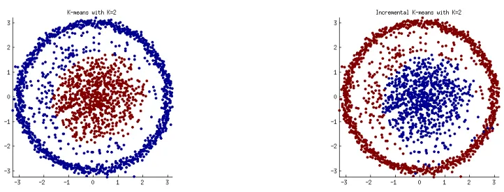
(a) Clusters using batch mode. Run time: 27.5 sec
(b) Clusters using incremental mode. Run time 6.4 sec
Figure 1: Result incremental diffusion maps
Incremental Diffusion map algorithm
Input:
D: distance matrix of size N ×N
T: distance matrix of new pointsN +p×p n: dimension of embedding
U,S,V : SVD of markov transition matrix Mt obtained using old points
Diffusion maps paramenets: σ, α
Output: U ,ˆ S,ˆ Vˆ, DD: Diffusion distance matrix of sizeN +p×N+p Steps:
1. Update D by adding new rows and columns from T to get ˆD(N +p×N +p)
2. Apply gaussian kernel to get W on ˆD
3. Compute new kernel by applying laplacian normalization,L(α)=D−αW D−α
4. CalculateM = (D(α))−1L(α)
5. Get new rowsR and columnsC from M
6. Get ˆU ,S,ˆ Vˆ by using update SVD procedure 2.2
7. Use ˆU ,Sˆto get new diffusion distance matrix DDt(i, j) = ||Ψt(xi)−Ψt(xj)||2
2.4
Results
using proposed incremental diffusion maps procedure. To simulate real world setting we update the embedding 10 points at a time, calling incremental update 40 time in this case. Once we get the final embedding after updating all 400 points for both batch and incremental setting we use k-means with k = 2 to visualize the effectiveness of diffusion distance learned. Final results are plotted in figures 1.
All the experiment was done on Sony machine with i3 processor and 4GB RAM. It can be observed that the results are very close with very less run time than batch mode. We have tested this methods on other datasets but due to high approximation error in markov matrix calculation and update svd procedure results are not appreciable.
2.5
Conclusion and future work
From our results we conclude that approximation in markov matrix and svd is not very appreciable, however, the current method used a basic svd update procedure and using recent advanced procedures [1] could lead to further improvements.
References
[1] Xilun Chen and K Selcuk Candan. “LWI-SVD: low-rank, windowed, incremental singular value decompositions on time-evolving data sets”. In: Proceedings of the 20th ACM SIGKDD international conference on Knowledge discovery and data mining. ACM. 2014, pp. 987–996.
[2] Ronald R Coifman and Stephane Lafon. “Diffusion maps”. In:Applied and computational harmonic analysis 21.1 (2006), pp. 5–30.
[3] Jason V Davis et al. “Information-theoretic metric learning”. In: Proceedings of the 24th international conference on Machine learning. ACM. 2007, pp. 209–216.
[4] M. Lichman. UCI Machine Learning Repository. 2013. url:http://archive.ics.uci. edu/ml.