Design and Control of UAV Systems: A Tri-Rotor UAV Case Study

Design and Control of UAV Systems:

A Tri-Rotor UAV Case Study

A thesis submitted to the University of Manchester for the degree of Doctor of Philosophy in the Faculty of Engineering and Physical Sciences

2012

Mohamed Kara Mohamed

Contents

Abstract 6

Declaration 7

Copyright Statement 8

Dedication 10

Acknowledgment 11

1 Introduction 12

1.1 Background and Motivation . . . 12

1.2 Thesis Structure and Outlines . . . 14

1.3 Publications . . . 16

2 Two Stage Feedback Linearisation To Handle Actuator Dynamics in Control

2.1 Introduction . . . 18

2.2 Review of Input Output Feedback Linearization . . . 19

2.3 Analyzing The Effect of Unmodeled Actuator Dynamics on Feedback Linearization . . . 23

2.4 New Two Stage Feedback Linearisation to Handle Actuator Dynamics . . . 32

2.5 Summary . . . 42

3 An Explicit Design Procedure for Propulsion Systems of Electrically Driven VTOL UAVs 43 3.1 Introduction . . . 44

3.1.1 Why A Design Procedure Is Needed? . . . 44

3.2 Electric Propulsion Systems . . . 46

3.2.1 Propellers . . . 47

3.2.2 Propeller Model Verification . . . 52

3.2.3 Electric Motors . . . 55

3.2.4 Electric Speed Controllers (ESCs) . . . 59

3.2.5 Battery Packs . . . 59

3.3 Design Methodology . . . 60

4 A New Cost Effective Indoor Navigation Technique for UAV Systems 66

4.1 Introduction and Related Work . . . 67

4.2 System Description . . . 69

4.3 Theoretical Formulation . . . 72

4.3.1 UAV Position . . . 72

4.3.2 UAV Orientation . . . 74

4.4 Implementation . . . 78

4.4.1 Obtaining the lengths of the Laser Beams . . . 79

4.4.2 Capturing The Laser Dots Coordinates . . . 80

4.4.3 On-board camera: restrictions to the angleα between the laser beams . . . 81

4.4.4 The Implementation Algorithm . . . 84

4.5 Summary . . . 85

5 Case Study: Design and Control of Novel Tri-Rotor UAV 87 5.1 Background and Motivation . . . 88

5.2 System Structure and Design . . . 90

5.3 Mathematical Modeling . . . 92

5.3.1 Reference Coordinate Systems and Notations . . . 92

5.4 Control System Design . . . 107

5.4.1 Control Synthesis Without Actuator Dynamics . . . 108

5.4.2 Analysis of Unmodeled Actuator Dynamics Effect . . . 119

5.4.3 Control System Design Including Actuators Dynamics: Compar-ison Study . . . 124

5.5 Propulsion System Design . . . 140

5.6 Hardware Assembly . . . 150

5.7 Summary . . . 152

6 Concluding Remarks 153 6.1 Contributions . . . 153

6.2 Directions for Future Research . . . 155

References 157

Abstract

The University of Manchester Mohamed Kara Mohamed Doctor of Philosophy

Design and Control of UAV Systems: A Tri-Rotor UAV Case Study 22 October 2012

Declaration

Copyright Statement

i. The author of this thesis (including any appendices and/or schedules to this thesis) owns certain copyright or related rights in it (the “Copyright”) and s/he has given The University of Manchester certain rights to use such Copyright, including for administrative purposes.

ii. Copies of this thesis, either in full or in extracts and whether in hard or electronic copy, may be made only in accordance with the Copyright, Designs and Patents Act 1988 (as amended) and regulations issued under it or, where appropriate, in accordance with licensing agreements which the University has from time to time. This page must form part of any such copies made.

iii. The ownership of certain Copyright, patents, designs, trade marks and other intel-lectual property (the “Intelintel-lectual Property”) and any reproductions of copyright works in the thesis, for example graphs and tables (“Reproductions”), which may be described in this thesis, may not be owned by the author and may be owned by third parties. Such Intellectual Property and Reproductions cannot and must not be made available for use without the prior written permission of the owner(s) of the relevant Intellectual Property and/or Reproductions.

iv. Further information on the conditions under which disclosure, publication and com-mercialisation of this thesis, the Copyright and any Intellectual Property and/or Re-productions described in it may take place is available in the University IP Policy1, in any relevant Thesis restriction declarations deposited in the University Library,

1_{see http://www.campus.manchester.ac.uk/medialibrary/policies/}

The University Library’s regulations2 and in The University’s policy on presenta-tion of Theses.

Dedication

To my parents and wife

Acknowledgment

All praise and thanks are due to Almighty Allah for his continuous blessing and for giving me the strength and ability to complete my PhD journey and write up this thesis.

I would like to thank my supervisor Dr. Alexander Lanzon for his support and readiness to help during the course of my research study. His suggestions and comments were always vital to polish and improve my research skills.

I must also thank my parents, Majed Kara Mohamed and Lutfia Kawusra who spent their lives educating and nurturing me until I have achieved my degrees and reached this level of the learning journey. Thanks my father and mother. I am grateful to have parents like you who cover me always with their love and support without a return.

I am also indebted to my wife Dima Kurbeh who joined me along the years of my PhD program. I thank her for taking care of our children and doing virtually all family chores on my behalf to give me spare times to stay at the university for long hours to read and research.

Chapter 1

Introduction

1.1

Background and Motivation

The field of robotic applications is no longer restricted to the area of conventional robot systems represented by programmed mechanical arms or complete human-like systems designed to do routine tasks and take limited decisions [1]. The robotic systems include now advanced designs of different vehicles with high capabilities to take hard decisions and operate in harsh circumstances [2]. In this regard, Unmanned Aerial Vehicles (UAVs) are considered highly advanced robotic systems and have seen unprecedented level of development and growth.

design and operation the most dynamic developing sector in aerospace industry [12, 3].

UAVs exist in various configurations and operate in different styles such as fixed-wing aircraft, rotary-wing or vertical take-off and landing (VTOL) with the latter being the rapidly evolving segment of all UAV markets [13]. In addition, VTOL systems are the major contributor in non-military applications [7]. Regardless of the type and application, the tendency shifts to smaller, more flexible, less costly and lighter weight UAV systems [14, 15, 16, 17] which leads to the emerge of miniature aerial vehicles (MAVs) and even micro UAVs in some projects that are referred to asµUAVs [18]. Furthermore, latest UAV

projects deploy multi-UAV systems to achieve more complex missions and cover wide operational areas [19, 20]. The multiple UAV operations benefit from the development of new technology in navigations systems, communication systems and control.

Designing and operating a UAV system is controlled by several factors such as the flight mechanics, mission type, vehicle instrumentations, on-board computing capability and the physical limitations of the vehicle [3, 21]. From research point of view, all these factors and other aspects of UAV systems are investigated and studied with an ultimate goal of improving the capability and stability of the vehicle, minimizing the power re-quirements and achieving full autonomy [9, 22]. With increasing number of research publications to meet these challenges and overcome the faced difficulties, open problems are still facing the design, control, application, navigation and sensors of UAV systems , see for example [3, 9, 23] and the references therein. Moreover, the rising of miniature air vehicles (MAVs) opens the door for more study related specifically to the design and development of these systems due to the limitation of size, weight and power of these miniature vehicles [18].

by introducing a novel cost-effective and easy to implement navigation strategy that ben-efits form computer vision algorithms. Furthermore, the thesis examines a novel design of tri-rotor UAV (in the sequel, referred to as the Tri-rotor UAV). The proposed UAV is used as a case study to demonstrate the effectiveness of the two stage feedback linearisa-tion where a centralizedH∞ controller associated with two stage feedback linearisation

is synthesized for the proposed Tri-rotor system. In addition, the propulsion system of the vehicle is designed using the proposed propulsion system design procedure. The Tri-rotor vehicle is constructed and prepared for the next stage of experimental studies and analysis.

The thesis can be seen as a general guideline that can be used in UAV projects involves designing and operating a UAV system from scratch. The various subjects conducted in the thesis are related to different aspects of UAV systems but they form in total a harmony of general issues one might encounter to design, operate and control a UAV system.

1.2

Thesis Structure and Outlines

The thesis is arranged into six chapters. Outlines of the main chapters of the thesis are as follows:

• Chapter 2: Two Stage Feedback Linearisation To Handle Actuator Dynamics in Control Systems for UAVs

• Chapter 3: An Explicit Design Procedure for Propulsion Systems of Electri-cally Driven VTOL UAVs

In this chapter, the design of propulsion systems for electrically driven VTOL UAVs is discussed. The design objectives are to generate sufficient thrust and obtain max-imum flight time by using the lightest possible components. Based on these factors, a design procedure is proposed to design efficiently electric propulsion systems from commercially available products. To implement the proposed procedure, a momentum theory based model is derived to quantify the thrust of propellers.

• Chapter 4: A New Cost Effective Indoor Navigation Technique for UAV Sys-tems

This chapter introduces a new cost-effective navigation system that can be used for indoor applications. The proposed system benefits partially from computer-vision navigation algorithms, but in the same time it is simple as there is no need for scene construction or full image matching algorithms which puts this algorithm ahead over other existing vision-based navigation systems. This fact is very important in mini UAVs where the size and power of on-board processors are limited. Moreover, the proposed system gives information about the position and orientation of the ve-hicle directly without the need for another integration, estimation or optimization stage which makes the system free from error accumulation.

• Chapter 5: Case Study: Design and Control of Novel Tri-Rotor UAV

procedure is motivated to design a linear controller for the system where a cen-tralizedH∞controller is synthesized to stabilize and track the translational motion

and rotational motion of the vehicle simultaneously. The goal was to completely build and operate the proposed Tri-rotor UAV using the synthesized controller. Un-fortunately, we ran out of time and this goal was not completely achieved within the time span of my PhD. The vehicle was built completely with installation of all equipment and components, yet, it is not ready for flight tests due to a technical communication problem between instruments. The results presented in this chapter are simulated using Matlab Simulink.

• Chapter 6: Conclusion

The conclusion and recommendations for future research are presented in this chap-ter.

1.3

Publications

Three conference papers were published based on the contents of this thesis as listed below. Parts of chapters 3 and 4 were presented in published conference papers 1 and 2 respectively. The conference paper 3 is based on Chapters 2 and 5.

1. Kara Mohamed, M., Patra, S. and Lanzon, A., “Designing simple indoor navigation system for UAVs”, Proceedings of The 19th Mediterranean Conference on Control and Automation , Corfu, Greece, pp. 1223–1228, June 2011.

2. Kara Mohamed, M., Patra, S. and Lanzon, A., “Designing electric propulsion sys-tems for UAVs”, Lecture Notes in Artificial Intelligence, Subseries of Lecture Notes in Computer Science, Vol. 6856, Springer, Proceedings of The 12th Annual Confer-ence Towards Autonomous Robotic Systems, Sheffield, UK, pp. 388–389, Septem-ber 2011.

Chapter 2

Two Stage Feedback Linearisation To

Handle Actuator Dynamics in Control

Systems for UAVs

This chapter is dedicated to the control design of UAV systems represented by nonlinear models. The chapter discusses feedback linearisation (FL) technique used to transform the UAV nonlinear system into a linear one and the effect of unmodeled actuator dynamics on the stability of the linearized system. A two stage feedback linearisation procedure to compensate actuator dynamics and linearize the UAV system is proposed.

2.1

Introduction

One of the common techniques used to handle nonlinear systems is to linearize the system by canceling the nonlinearly and then a linear system control method can be used to syn-thesize a controller for the linearized system [24]. Canceling the nonlinearity of nonlinear systems via feedback is known as feedback linearisation and it can be either state-input feedback linearisation or input-output feedback linearisation. Generally speaking, UAVs are nonlinear systems and input-output feedback linearisation is widely applied in UAV systems [25, 26, 27, 28] where it can be viewed as a method to transform the UAV non-linear system into a non-linear system with respect to a new defined control input.

To simplify the implementation of feedback linearisation, several assumptions related to the model of the system and its operating point are considered. Among these assump-tions is the negligence of actuator dynamics. In UAV literature, actuator dynamics are commonly neglected when modeling the system and synthesizing a controller, see for example [29, 30, 31] and the references therein. In these references, it is assumed that actuators are fast and their dynamics can be neglected safely. In this chapter, we show that this assumption is not valid always and when it comes to feedback linearisation, un-modeled actuator dynamics have vital effect and they can destabilize the system.

2.2

Review of Input Output Feedback Linearization

This section outlines the input-output feedback linearisation method used to transfer a nonlinear system into a linear one and thereafter a linear control method can be used to synthesize a controller for the linearized system.

Consider a class of continuous multi-input multi-output (MIMO) nonlinear fully actuated UAV systems of the form:

˙

x= f(x) +

m

∑

j=1

g_j(x)u_j (2.1)

y=h(x) (2.2)

wherex∈_Rn _{is the state vector of the system,u}

j∈Ris the jth control input. y∈Rm is

the measured output vector of the system.

Assuming that f(·),h(·)andg_j(·)are sufficiently smooth in a domain_Dj⊂R, the

deriva-tivekof an outputy_i∈yis given by:

y(_ik)=Lk_fh_i+ m

∑

j=1

L_gjLk_f−1h_iu_j, 1≤i≤m, (2.3)

whereL_fhiis the Lie derivative of the scalar functionhiwith respect to the vector function

f and is defined as [35]:

L_fh_i(x) =∂hi(x)

∂x

f(x) (2.4)

and for higher derivatives, we have:

L2_fhi(x) =

∂ Lfhi(x)

∂x f(x)

.. .

Lk_fh_i(x) =

∂

Lk_f−1hi(x)

and similarly, we have:

L_gjL_fh_i(x) =∂ Lfhi(x)

∂x gj(x) = ∂

∂x

∂hi(x)

∂x f(x)

g_j(x)

.. .

L_gjLk_fh_i(x) = ∂

∂x

Lk_f−1h_i(x)f(x)g_j(x)

In order to understand how the inputu enters the linearized system, the notion "relative

degree" is introduced. From Eq. (2.3), the outputyiis said to have a relative degreeriif:

Lgjhi=LgjLfhi=LgjL

2

fhi=...=LgjL ri−2

f hi=0 ∀1≤i,j≤m (2.5)

whereL_gjh_iis the Lie derivative of the scalar functionh_iwith respect to the vector function

g_jand it is defined in similar way to the definition in Eq. (2.4) as:

Lgjhi(x) =

∂hi(x)

∂x gj(x)

and for higher derivatives, we have:

Lk_gjhi(x) =

∂

Lk_g−1

j hi(x)

∂x gj(x)

In this context, the relative degree can be seen as the number of times the output needs to be differentiated before the input appears explicitly. In LTI systems, the relative degree is defined as the difference between the number of poles and the number of zeros of the system. In our case, the total relative degree of the MIMO system (2.1) - (2.2) in _D is defined as the sum of the relative degree of all outputs:

r=r1+r2+...+rm (2.6)

dynam-ics are dynamdynam-ics related to these unobservable states. These unobservable states might be unbounded and destabilize the system. When the relative degree of the system equals to the number of states, all states will be observable and there is no internal dynamics. For now, let’s assume thatr=nwith no internal dynamics.

Define a new mappingζ =T(x)as:

ζ =       ζ1 ζ2 .. . ζm       , (2.7) where

ζi=      

h_i(x)

L_fh_i(x) .. .

Lri−1

f hi(x)      

, 1≤i≤m. (2.8)

We define also a new input vectorϑ as:

ϑ =      

y(₁r1) y(r2)

2 .. .

y(mrm)       (2.9)

Then, the nonlinear system (2.1) - (2.2) can be transformed into a linearized system of a global normal form defined by:

˙

ζ =AAAcζ+BBBcϑ (2.10)

where

A

AA_c=

     

AAA1

AAA2 . ..

A AA_m

     

, BBB_c=       B1 B2 . .. B_m      

, CCC_c=       C1 C2 . .. C_m      

A_j,B_j,C_jwith 1≤ j≤mare the matrices of the Brunovsky canonical form and given by [36]:

A A

A_j=

        

0 1 0 0 · · · 0 0 0 1 0 · · · 0

..

. ... ... ... ... ... 0 0 0 · · · 0 1 0 0 0 0 · · · 0         

∈_Rrj×rj_,B j=       0 .. . 0 1      

∈_Rrj×1_,C j=

h

1 0 · · · 0 i

∈_R1×rj

(2.12)

The feedback linearisation law from system (2.1) (2.2) to the linearized system (2.10) -(2.11) is given by:

u(x,ϑ) =α(x) +βββ−1(x)ϑ (2.13)

where

βββ(x) =



  

L_g1Lr1−1

f h1(x) · · · LgmL r1−1

f h1(x) ..

. ... ...

L_g1Lrm−1

f hm(x) · · · LgmL rm−1

f hm(x) 

  

, (2.14)

α(x) =−βββ(x)−1



  

Lr1

f h1(x) .. .

Lrm

The matrix βββ(x) in Eq. (2.14) is called the decoupling matrix. We assume that β is

invertible on the domain_Dand then we define the feedback linearisation on this domain.

The linear system represented by Equations (2.10) - (2.11) can be controlled using a linear system control method whereas the field of linear systems is rich of several control methods that can be used to stabilize the system and track the reference signals, e.g., LQR, LQG, state feedback andH_∞loop-shaping design [37, 38]. In this thesis, we invoke the H∞ loop-shaping design as a robust control method for the linearized system when

considering the case study of the Tri-rotor UAV. The motivation behind the H∞

loop-shaping design along with a brief introduction of the procedure is presented Chapter 5.

2.3

Analyzing The Effect of Unmodeled Actuator

Dynam-ics on Feedback Linearization

The input-output feedback linearisation technique presented in the previous section lin-earizes the UAV nonlinear system by canceling the nonlinearities via feedback lineari-sation. In UAV systems, when applying feedback linearisation, actuator dynamics are usually neglected assuming that actuators are fast enough to apply the required con-troller action without a considerable delay, see for example [29, 30, 31] and the references therein. In practice, the inpututo the UAV system (2.1) - (2.2) is applied by mechanical or electrical actuators of physical constraints which makes the assumption of ignoring their dynamics questionable. In this section, we analyze the effect of unmodeled actuator dynamics on input-output feedback linearisation.

We assume that actuator dynamics can be approximated by a MIMO LTI system as:

˙

xa=AAAaxa+BBBaua (2.17)

y_a=CCC_ax_a (2.18)

wherex_a∈_Rna _{is the state vector of the actuators system andu}

a∈Rmis the control input

valuesx_a∈_D, where_Dis the domain of existence of the feedback linearisation law.

We recall the linearized system of the nonlinear model (2.1) - (2.2) which is given by:

˙

ζ =AAAcζ+BBBcϑ (2.19)

y=CCCcζ (2.20)

and the feedback linearisation law from (2.13) is:

u(x,ϑ) =α(x) +βββ−1(x)ϑ (2.21)

Suppose that the mappingζ =T(x)is invertible and we can get:

x=T−1(ζ) (2.22)

Using Eq. (2.21) and the mapping (2.22), the artificial control input ϑ in terms of the

physical inputucan be given by:

ϑ(ζ,u) =βββ(ζ)(u−α(ζ)) (2.23)

The linearized system can be written in terms of the physical input as:

˙

ζ =AAAcζ+BBBcβββ(ζ)(u−α(ζ)) (2.24)

y=CCC_cζ (2.25)

represented by:

˙

ζ =AAAcζ+BBBcβββ(ζ)(ya−α(ζ)) (2.26)

˙

x_a=AAA_ax_a+BBB_au (2.27)

y_a=CCC_ax_a (2.28)

y=CCC_cζ (2.29)

Using (2.21) the mapping (2.22), we write the system fromϑ toyas:

˙

ζ =AAAcζ+BBBcβββ(ζ)CCCaxa−BBBcβββ(ζ)α(ζ) (2.30)

˙

x_a=AAA_ax_a+BBB_aα(ζ) +BBBaβββ−1(ζ)ϑ (2.31)

y=CCCcζ (2.32)

The perturbed system (2.30) - (2.31) by actuator dynamics is nonlinear system and dif-ferent from the linearized system (2.10) - (2.11). The order of the perturbed system from

ϑ toy isn+nawhere nis the order of the UAV system without actuators and na is the order of the actuators system. There is no guarantee that the synthesized controller for the linearized plant (2.10) - (2.11) will be able to control the nonlinear system (2.30) - (2.31) and if the controller manages to stabilize the nonlinear system (2.30) - (2.31), apparently the performance will be deteriorated. Therefore, actuators dynamics cannot be neglected safely always when using feedback linearisation and they show risk of destabilizing the overall system.

Example 1. To demonstrate the effect of unmodeled actuator dynamics on feedback

lin-earisation, we consider a small example of nonlinear system and try to synthesize different controllers while studying the effect of unmodeled actuator dynamics at each case.

Consider the SISO nonlinear system given by:

˙

x₁=x₂ (2.33)

˙

x₂=x₁x₂+x2₁+u (2.34)

We linearize the system using input-output feedback linearisation. Therefore, we have:

˙

y=x˙₁=x₂ (2.36)

¨

y=x˙₂=x₁x₂+x2₁+u (2.37)

The relative degree of the system(r=2)equals to the order of the system (n=2)and there is no internal dynamics. To linearize the system we choose:

¨

y=ϑ. (2.38)

Then, we haveα(x) =−x1x2−x2₁andβ(x) =1. The feedback linearisation law is:

u=ϑ−x1x2−x21. (2.39)

The linearized system fromϑ toyis a double integrator system given by:

" ˙

ζ1 ˙

ζ2 #

= "

0 1 0 0

# "

ζ1

ζ2 #

+ "

0 1 #

ϑ (2.40)

y=h1 0

i "

ζ1

ζ2 #

(2.41)

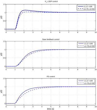
We invoke now different controllers for the linearized system and observe the effect of unmodeled actuator dynamics in each case. Table 2.1 summarizes the used controllers and the transfer functions of the controller for each case.

Linearized Plant P(s) Controller Synthesis method

0.54s3+4.5s2+4.75s+1.31

0.001s4_+0.034s3_+0.43s2_+1.83s+1.08 H∞loop shaping design

1/s2 k1=12,k2=35,kI=30 State feedback with integrator

k_d=8.75,kp=10 PD

The step responses of the linearized system using the specified controllers are summarized in Figure 2.1.

0 1 2 3 4 5 6 7 8 9 10

0 0.5 1 1.5

y(t)

H

∞ LSDP control

0 1 2 3 4 5 6 7 8 9 10

0 0.5 1 1.5

y(t)

State feedback control

0 1 2 3 4 5 6 7 8 9 10

0 0.5 1 1.5

y(t)

time (s) PD control

Figure 2.1: Step responses of the nonlinear system using input-output feedback linearisa-tion associated with the specified controllers without considering actuator dynamics

To study the effect of unmodeled actuator dynamics on feedback linearisation, we con-sider a SISO LTI actuator system given by:

˙

x_a=−1

t_axa+

1

t_aua (2.42)

where t_a is the time constant of the actuator system and it indicates the speed of the actuator.

To impose the unmodeled actuator dynamics on the linearized system we have the map-ping:

x₁=ζ1 (2.44)

x₂=ζ2 (2.45)

and then we have the perturbed plant as:

˙

ζ1=ζ2 (2.46)

˙

ζ2=xa+ζ1ζ2+ζ12 (2.47)

˙

x_a=−1

ta

x_a+ 1

ta

(−ζ1ζ2−ζ12) + 1

ta

ϑ (2.48)

y=ζ1 (2.49)

0 0.5 1 1.5 2 2.5 3 −1

0 1 2 3 4

H_∞ LSDP control

y(t)

0 1 2 3 4 5 6 7 8 9 10

0 0.5 1 1.5 2

State feedback control

y(t)

0 1 2 3 4 5 6 7 8 9 10

−2 0 2 4

PD control

y(t)

time (s)

t

a=0.1s

t

a=0.2s

t

a=0.3s

t_a=0.4s

t

a=0.5s

t

a=0.1s

t_a=0.2s

t

a=0.3s

t_a=0.4s

t

a=0.5s

t

a=0.1s

t_a=0.2s

t

a=0.3s

t

a=0.4s

t_a=0.5s

Figure 2.2: Step responses of the linearized system under the effect of first order unmod-eled actuator dynamics.

It can be seen from Figure 2.2 that in case of the H∞ control and the PD controller,

the state feedback control with integrator, unmodeled actuator dynamics deteriorate the performance regardless of the speed of the dynamics.

For further analysis of the negative impact of actuator dynamics on feedback linearisation, we consider second order actuator dynamics as:

˙

x_a1 =x_a2 (2.50)

˙

x_a2 =−1

ta

x_a2+ 1

ta

u_a (2.51)

y_a=x_a1 (2.52)

Figure 2.3 shows the response of the system when imposing unmodeled second order ac-tuator dynamics. In this case, the synthesized controllers fail to accommodate the acac-tuator dynamics and the system becomes unstable regardless of how fast actuators are.

0 0.5 1 1.5 2 2.5 3 −1

0 1 2 3 4

H_∞ LSDP control

y(t)

0 0.2 0.4 0.6 0.8 1 1.2 1.4 1.6 1.8

0 0.5 1 1.5 2

State feedback control

y(t)

0 0.2 0.4 0.6 0.8 1 1.2 1.4 1.6 1.8

0 2 4 6

PD control

y(t)

time (s)

t

a=0.1s

t

a=0.2s

t

a=0.3s

t_a=0.4s

t_a=0.5s

t_a=0.1s

t_a=0.2s

t_a=0.3s

t

a=0.4s

t

a=0.5s

t

a=0.1s

t

a=0.2s

t

a=0.3s

t

a=0.4s

t

a=0.5s

2.4

New Two Stage Feedback Linearisation to Handle

Actuator Dynamics

The previous section shows the negative effect of unmodeled actuator dynamics on sys-tem performance when implementing feedback linearisation. In this section, we develop a two stage feedback linearisation algorithm to compensate actuator dynamics and maintain the validity of the linear control associated with feedback linearisation for the nonlinear system. In the proposed two stage algorithm, the first stage handles actuator dynamics using inner loop linearisation/compensation while the second stage is to design the outer loop and linearize the main nonlinear system. Compared with the direct way of includ-ing actuator dynamics in the overall system before implementinclud-ing feedback linearisation, the proposed two stage algorithm simplifies the implementation of feedback linearisation and minimize the effect of actuators system uncertainty on the stability of the linearized system.

Assuming that the model of actuators system is available, consider a nonlinear MIMO fully actuated system represented by:

˙

x= f(x) +GGG(x)u (2.53)

y=h(x) (2.54)

and a nonlinear actuators system given by:

˙

x_a= f_a(x_a) +GGG_a(x_a)u_a (2.55)

ya=ha(xa) (2.56)

wherexa∈Rna andya,ua∈Rm. f(·), fa(·)andh(·),ha(·)as well as the column vectors of

G

GGandGGGaare assumed sufficiently smooth in the domainsD,Da⊂Rrespectively where

the matricesGGGandGGGaare given by:

GGG=hg1 g2 · · · gm i

, (2.57)

G

GG_a=hga1 ga2 · · · gam i

The complete nonlinear system including actuator dynamics can be represented by:

˙

x= f(x) +GGG(x)y_a (2.59)

y=h(x) (2.60)

and

˙

xa= fa(xa) +GGGa(xa)ua (2.61)

y_a=h_a(x_a) (2.62)

(2.63)

We propose now two stage feedback linearisation algorithm to linearize the nonlinear UAV system . In the first stage, we linearize and control the actuator system assuming that actuators states are available, the actuators system has a well-defined relative degree ofraand the dynamics of the actuators are invertible. We linearize the nonlinear actuator system by defining the feedback linearisation law for the actuator system as:

ua=αa+βββ−_a1ϑa (2.64)

with αa and βββ_a are defined respectively as in Eq. (2.15) and (2.14) with regard to the

actuators nonlinear system. The inputϑais defined as:

ϑa= 

     

y(ra1)

a1

y(ra2)

a2

.. .

y(armam) 

     

(2.65)

where

y(_ar_iai)=Lr_fai

ahai+ m

∑

j=1

L_g

a jL r_ai−1

fa haiuaj, 1≤i≤m. (2.66)

and

Now, the linearized actuators system can be represented by:

˙

ζa=AAAaζa+BBBaϑa (2.68)

y_a=CCC_aζa (2.69)

such asAAAa,BBBa,CCCaare defined according to Eq. (2.12) with regard to the actuators system.

ζais a new actuator state vector defined throughout the mappingζa=Ta(xa).

System (2.68) - (2.69) is a MIMO decoupled system in which each channel can be handled individually.

We consider now the SISO System of theithactuator channel. We have:

ζai=       h_i ˙ h_i .. .

h(_irai)

      =      

ζi1

ζi2

.. .

ζi(_rai−1)       (2.70)

and therefore we can write the dynamics of the theith channel as:

˙

ζi1=ζi2 (2.71)

˙

ζi2=ζi3 (2.72)

..

. (2.73)

˙

ζi(_rai−1)=ϑai (2.74)

y_ai=ζi1 (2.75)

where 1≤i≤m.

y_di=u_i. We define a new strict feedback error systems as:

e_i1 =ζi1−ui (2.76)

e_i2 =ζi2−zi1−u˙i (2.77)

..

. (2.78)

e_i

rai =ϑai−zi(_rai−1)−u

(r_ai−1)

i (2.79)

wherez_ik, 1≤k≤r_ai−1 is a Backstepping control law that is used to achieve stability and convergence of the overall error system. We design z_ik using Lyapunov functionV_ik

such that ˙Vik is semidefinite. Following [39],zik can be designed as:

z_ik =−e_ik−1−c_ike_ik+

k−1

∑

j=1

∂zi(j−1)

∂ ζij

ζi(j+1)+

∂zi(j−1)

∂u(_ij−1)

u(_ij)

!

(2.80)

The candidate for the Lyapunov function is:

V_ik =V_ik−1+1

2e 2

ik (2.81)

withVi1 =e

2 i1.

The final control law for theithchannel is:

ϑai =zi(rai−1)+u

(r_ai)

i (2.82)

and that leads to:

˙

V_i

rai =− r_ai

∑

j=1

c_ije2_i

j ≤0 (2.83)

The resulting error system for theithchannel is:



  

˙

e_i1

.. . ˙

ei_rai     =      

−ci1 1 0 · · · 0

−1 −ci2 1 · · · 0

0 −1 . .. ... ... 0 0 · · · −1 −c_i

rai          

e_i1

.. .

ei_rai 

  

The error system in Eq. (2.84) is globally uniformly stable at equilibrium e_i=0 and limt→∞ei(t) =0 which means that the global asymptotic tracking is achieved, whereeiis defined as:

e_i=



  

e_i1

.. .

e_i

rai 

  

(2.85)

The proof can obtained easily using Lyapunov theory. The transient performance of the error system can be controlled by the design parametersc_ik. In general, increasingc_ikwill improve the transient performance of the error system [39].

We repeat the previous Backstepping tracking design for all actuator channels, i.e., 1≤

i≤m, and finally we have:

ϑa(Ta(xa),u,u˙,u¨,· · ·,u(a1),· · ·,u(am)) = 

  

ϑa1

.. .

ϑam 

  

(2.86)

The design of the inner loop ensures thaty_a converges touasymptotically for all initial values.

Assuming that the inner loop has high and sufficient bandwidth, we can put y_a≈uand then we can now perform the second stage by implementing input-output feedback lin-earisation of the main nonlinear system using the standard procedure described in Section 2.2. Figure 2.4 represents a block diagram of the developed two stage feedback linearisa-tion for nonlinear systems including actuator dynamics.

dynam-Stage One: Actuator Compensation

Actuators System

UAV System y

a

ϑ

and Linearization

ϑ u Compensator ua

a

x

x

a

y UAV

System FL

Figure 2.4: Block diagram of the proposed two stage feedback linearisation.

ics can be written as a two cascaded nonlinear system:

˙

x= f(x) +GGG(x)h(x_a) (2.87)

˙

xa= fa(xa) +GGGa(xa)ua (2.88)

y=h(x) (2.89)

System (2.87) - (2.88) can be linearized as one system using standard feedback linearisa-tion. However, this method is complex and requires derivation along both vector statesx_a

andx, which means that the vector functions f(·),g_i(·), f_a(·)andg_ai(·)need to be smooth and diffeomorphic up to the leveln+n_a. A comparison study between the proposed two stage feedback linearisation and the standard linearisation of the whole system will be conducted when considering the example of Tri-rotor UAV in Chapter 5.

To demonstrate the proposed linearisation algorithm, we consider again Example 1 and apply the proposed two stage feedback linearisation procedure.

Stage 1 We consider in this stage the actuator dynamics given in (2.50) -(2.52). The goal is to design an inner loop feedback controller so thaty_atracks the reference signal

u. We define the new error states as:

e₁=x_a1−y_d (2.90)

e2=xa2−z1−y˙d (2.91)

and then we have the error system as:

˙

e₁=x˙_a1−y˙_d (2.92) ˙

e₂=x˙_a2−z˙₁−y¨_d (2.93) (2.94)

We have from the dynamics of the system:

˙

x_a1 =x_a2 (2.95)

˙

x_a2 =−1

ta

x_a2+ 1

ta

u_a (2.96)

Therefore, the error system is:

˙

e₁=x_a2−y˙_d (2.97)

˙

e2=−

1

t_axa2+

1

t_aua−z˙1−y¨d (2.98)

We have from Eq. (2.91):

˙

and therefore:

˙

e₁=x_a2−(−e₂+x_a2−z₁) (2.100)

=e₂+z₁ (2.101)

˙

e2=−

1

t_axa2+

1

t_aua−z˙1−y¨d (2.102)

We define a Lyapunov function:

V₁= 1

2e 2

1 (2.103)

whose derivative is:

˙

V₁=e₁e˙₁ (2.104)

=e1(e2+z1) (2.105)

Then, we choose:

z1(x1) =−c1e1 (2.106)

withc1>0 a design parameter. Then, we have:

˙

V1=−c1e21+e1e2 (2.107)

The terme₁e₂will be canceled in next step.

Let us now consider the equation:

˙

e₂=−1

t_axa2+

1

t_aua−z˙1−y¨d (2.108)

We define a Lyapunov function:

V₂=V₁+1

2e 2

whose derivative is:

˙

V₂=V˙₁+e₂e˙₂ (2.110)

=−c₁e2₁+e₁e₂+e₂(x˙_a2−z˙₁−y¨_d) (2.111)

=−c1e21+e1e2+e2(− 1

t_axa2+

1

t_aua−z˙1−y¨d) (2.112)

Then, we choose the control input as:

u_a=t_a(−c₂e₂−e₁+z˙₁+y¨_d+ 1

ta

x_a2) (2.113)

withc2a positive design parameter, and this gives:

˙

V2=−c1e21−c2e22≤0 (2.114)

We have:

˙

z₁=−c₁e˙₁ (2.115)

=−c₁(e₂+z₁) (2.116)

and therefore the control law is given by:

u_a=t_a

−(c₁+c₂− 1

t_a)xa2−(c1c2+1)xa1+ (c1c2+1)yd+ (c1+c2)y˙d+y¨d

(2.117)

We choosec₁andc₂high enough to guaranteey_a≈u.

stage 2 This stage includes the feedback linearisation of the original system (2.33) -(2.34) neglecting actuator dynamics. Eq. (2.39) gives the feedback linearisation law of the outer loop in regard to the main nonlinear system.

0 1 2 3 4 5 6 7 8 9 10 0

0.5 1 1.5

y(t)

H_∞ LSDP control

0 1 2 3 4 5 6 7 8 9 10

0 0.5 1 1.5

y(t)

State feedback control

0 1 2 3 4 5 6 7 8 9 10

0 0.5 1 1.5

y(t)

time (s)

PD control

c1,c2 >100 c1=70,c2=50

c1,c2 >100 c1=70,c2=50 c1,c2 >100 c1=70, c2=50

The graphs depicted in Figure 2.5 shows that with large value of c₁ and c₂ the perfor-mance of the system is typical to the nominal plant without actuators shown in Figure 2.1. The compensation of the actuator dynamics using the proposed two stage feedback linearisation succeeds to maintain the validity of the feedback linearisation for the main nonlinear system without actuators.

2.5

Summary

Chapter 3

An Explicit Design Procedure for

Propulsion Systems of Electrically

Driven VTOL UAVs

This chapter proposes a systematic design procedure for electric propulsion systems of VTOL UAVs based on the design specifications that are given in terms of the required thrust, permissible weight of the propulsion system and required flight time. The solution space of the proposed design methodology is a subset of commercially available products, which enhances the applicability of the procedure to the practicing community. For the purpose of the proposed design procedure, we introduce a mathematical model for the thrust and mechanical power of fixed pitch propellers.

3.1

Introduction

A key part of UAV systems is the propulsion system that generates the required lifting force for all flying modes; i.e., taking-off, hovering, forward flying, maneuvering and landing. In practice, different types of propulsion systems exist, and the selection of best suitable system depends on many factors such as the vehicle size and structure, the op-erational environment, the payload and flight time of the vehicle [40, 41]. Therefore, for different UAV designs and applications, designers choose different propulsion systems; e.g., electric propulsion systems, jet engines or reciprocating piston engines. Due to their advantages, electric propulsion systems are widely used in UAV systems and particularly in mini UAVs and research platforms [41, 40, 42, 43]. The advantages and disadvan-tages of electric propulsion systems are summarized in [40]. The advandisadvan-tages of electric propulsion systems are inherited from electric motors that are reliable and can be con-trolled easily. Moreover, electric motors are less noisy, require less maintenance and have no emissions compared to jet and internal combustion (IC) engines. On the other side, electric propulsion systems reports some disadvantages due to sensitivity to water and conductive liquids. Another point in the negative side of propulsion systems is related to electric batteries. The energy of electric batteries is still far shorter than that of liquid fuels, which results in shorter flight time. However, the available electric batteries have adequate power capacities for short-flight missions and demonstration purposes. Never-theless, electric propulsion systems are still dominant in small UAV systems and research platforms. This in turn calls for more focusing on the design and operation of electric propulsion systems.

3.1.1

Why A Design Procedure Is Needed?

like the radius and pitch angle of the propeller and the air density as will be shown later in Section 3.2.1.

Due to the considerable relative weight of electric batteries and motors compared to other components of UAV systems, the chosen electric propulsion system has an impact on the total weight of the vehicle which in turn affects the payload capability and the maneuver-ability of the UAV. Moreover, the power consumption of electric motors and the capacity of electric batteries are important factors in specifying the flight time of the UAV. There-fore, the chosen electric propulsion system needs to be designed effectively in order to improve the thrust-to-weight ratio of the system and decrease the weight of the vehicle. This in turn enhances the payload capability, the maneuverability and the operational flight time of the UAV.

packages to design electric propulsion systems [51, 52]. In these softwares, a routine is used to analyze the supplied specifications of the UAV, and then suggests a set of com-ponents to construct the required electric propulsion system. However, the algorithms of these software are ambiguous and the suggested components do not always exist commer-cially in the market. As a result, a global search is followed to obtain the best matching existing alternative products which might deviate from the optimal solution.

In this chapter, a systematic design procedure is proposed to select the components of electric propulsion systems for VTOL UAVs. Prior to the design steps, the technical specifications of each component are discussed in detail and a mathematical model for the propeller thrust that is explicit and easy to use for design purposes is derived. In the proposed design strategy, two goals are considered: one is to increase the payload capacity of the UAV by reducing the total weight of the propulsion system. The other goal is to increase the flight time by choosing the best possible battery pack.

3.2

Electric Propulsion Systems

Eneregy

Storage

Unit

Electronic

Speed

Controller

(ESC)

Electric

Motor

(BLDC)

Propeller

Figure 3.1: Structure and elements of an electric propulsion unit.

requirements of sufficient static thrust for taking off and hovering, minimum power con-sumption to generate the required thrust, minimum weight of the propulsion system, and maximum flight time [53]. These design parameters are reflected directly by the speci-fications of the components of the constructed electric propulsion system . For instance, the size, shape and rotational speed of the propeller determine the maximum thrust it can generate. The constants of the electric motor specify the maximum torque and rotational speed that can be produced at the shaft and these should match with the propeller re-quirements to generate the specified thrust. The electric capacity of the battery should be sufficient to operate the motor at the specified rotational speed for the required flight time while in the same time the size and weight of the battery should fit the structure and design of the vehicle. In the following subsections, the principle components of electric propulsion systems and the important design factors of each component are highlighted. Side by side, the technical specifications of each component along with the mathematical model that represent the component is illustrated to make the design steps easy to use for the practicing community.

3.2.1

Propellers

accurate mathematical model for the developed thrust by air propellers [54, 55, 56]. In general, the available thrust and power models, e.g. the blade element model, need an exact description of the geometric shape of the propeller in order to obtain the thrust and power coefficients required to derive the thrust model. In the market of model aircraft and mini UAVs, the geometric descriptions of available propellers are not available and the power/thrust coefficients are not supplied. An alternative way to get the missing informa-tion is to use wind tunnel experiments to extract the thrust curves of the given propeller(s) [57, 46]. The wind tunnel experiment is not always available or easy to perform, and therefore, an explicit mathematical thrust model that requires less information about pro-pellers is useful. The methodology adopted in this chapter is to use the simplest possible model to bring the design to the neighborhood of the optimized choice of components as it is futile to require experiments or design methods that cannot be possibly imple-mented in practice. In this section, a new mathematical model of air propellers based on [54, 55, 56] is derived. This model is used latter in Section 3.3 to develop the proposed design procedure for electric propulsion systems of VTOL UAVs.

Using the momentum theory [55] while considering propellers as actuator disks and with the following assumptions: (i) ideal fluid (air in this case) with no energy dissipation through friction or energy transfer to the ideal fluid, (ii) no viscosity and compressibility of the air and (iii) no elastic bending of the propellers, the static thrust f_pdeveloped by a propeller pis given as:

f_p=2µaApυa2, (3.1)

whereµa is the air density,Ap=πR2pis the disk area of the propeller,Rpis the radius of the propeller andυais the induced velocity of the incoming air by the propeller.

For constant pitch propellers and uniform airflow, the induced velocity is given by:

υa=κpωpRp, (3.2)

approximated [56] as:

κp=

σpk1 16

"s

1+ 64 3σpk1

θp

−1 #

, (3.3)

whereθpis the pitch angle of the propeller,k1is known as the two-dimensional lift slope factor1andσpis the solidity factor that is defined by:

σp=

blade area disk area =

n_pd_pR_p

πR2_p =

n_pd_p

πRp

, (3.4)

wheren_pis the number of blades of the propeller andd_prepresents the chord length of the blade. For a propeller with varying chord length,dpis taken as the average chord length of the blade. By using Equations (3.2) - (3.4), the generated thrust can be written as:

fp=

µa

128π

n2_pd2_pk₁2 R2_p

!

ω_p2R4_p

s

1+ 64πRp 3npdpk1

θp

−1 !2

. (3.5)

For simplicity of representation, a new variableC_pis defined as a function of the number of bladesnp, the chord-to-radius ratiodp/Rpand the pitch angleθp:

C_p= dp

Rp    v u u u t 

1+ 64π 3n_pdp

Rpk1 θp



−1 



. (3.6)

UsingC_p, the developed thrust f_pcan be written as:

f_p= µan

2 pk12 128π ω

2

pR4pC2p. (3.7)

Using Eq. (3.7), one can calculate the thrust f_p generated by a propeller p of radiusR_p

and pitch angle θp when rotating at rotational speed ωp. Assuming that Cp is radius independent due to the fact that the ratiod_p/R_pcan be considered constant for a family of propellers2, the radius of the propeller has more effect on the generated thrust than other

1_{In this thesis,k}

1is assumed constant with a value ofk1=5.7 [56].

2_{As the radius of the propeller increases, the average chord length increases in the same rate and hence}

variables: f_p∝R4_p. In addition, Eq. (3.7) can be used to calculate the rotational speed

necessary to generate a given thrust f_p by a propeller of radiusR_pand pitch angleθp as following:

ωp= s

fp

R4

pC2p

128π

µan2pk12

. (3.8)

An experiment based validation is conducted in next section to test the validity of the thrust model represented by Eq. (3.7).

In order to generate the required thrust fp, an external mechanical power Pfp is needed (supplied by a motor) to rotate the propeller at the particular rotational speed ωp. Fol-lowing the momentum theory, this mechanical power is defined as the power needed to overcome the drag torque and mathematically is given by [54]:

P_fp =2µaAp(υ∞+υa)2υa, (3.9)

whereυ∞is the air speed in the direction of the propeller. µa, Ap andυa are defined as in Eq. (3.1). For static thrust, the directional speed of the air toward the propeller is zero; i.e.,υ∞=0, and then Eq. (3.9) is simplified to:

P_fp =2µaApυa3. (3.10)

Using Equations (3.2) - (3.4) yields:

P_fp = µa

2048π2(npk1)

3

(ωpCp)3R5p. (3.11)

For a given propeller p, the termωpCp can be obtained from Eq. (3.7) as a function of the generated thrust f_pand the radiusR_p, and then substituted into Eq. (3.11) to give the relationship between the thrust fpand the powerPfp required to generate this thrust:

P_fp= √ 1

2µaπ (f_p)32

Rp

. (3.12)

as it involves only few variables; the propeller radius and air density. For instance, to calculate the power that is necessary to generate a specific thrust f_p, the designer needs only to know the radius of the propeller and the air density.

Pitch Length vs. Pitch Angle

Broadly speaking, the pitch of commercial propeller available in the market is specified in terms of pitch lengthβp rather than pitch angleθp. The pitch length is defined as the distance that the propeller would move forward in each revolution without slipping [54]. However, in order to use Eq. (3.7) or Eq. (3.11) to calculate the developed thrust f_p or the powerP_fp, the pitch angle must be known a priori for obtainingC_p(see Eq. (3.6)). In twisted propellers, the pitch angle and pitch length vary along the radiusr, whereris the distance from the center of the propeller to the point of measurement,i.e., 0≤r≤Rp. The relationship between the pitch lengthβ(r)and the pitch angleθ(r)at a radiusris given

by:

β(r) =2πrtan(θ(r)). (3.13)

For constant-pitch length propellers3, the pitch length is constant along the radius, i.e., the pitch angleθ(r)decreases asrincreases so that the pitch lengthβ(r)remains fixed along

the radius span. Empirically, it was shown in [56] that for the case of constant pitch length propellers, the pitch angle at the radiusr=0.75R_pis sufficient to be used to calculate the generated thrust of the propeller. Therefore,θpis obtained as following:

θp=θ(0.75Rp) =arctan

2βp 3πRp

, (3.14)

whereβpandRpare known.

For the purpose of propulsion systems design, a simplified propeller model is necessary to get a quantitative measure of important physical quantities, e.g. thrust and power, and the relationships between them. In this section, Eq. (3.7), Eq. (3.11) and Eq. (3.12)

3_{In this thesis, propellers are assumed to be constant pitch length (shortly called constant-pitch}

fulfill this objective easily when the propeller’s radius and pitch angle are known a priori. However, the proposed design procedure is similarly applicable for any other advanced propeller model available in hand.

3.2.2

Propeller Model Verification

The propeller model shown in the previous section is based on an assumption of constant inflow and incompressible air. In practice, these assumptions might be questionable. In order to verify the derived model and show that it is adequate for the design purpose, an experiment has been conducted to compare the actual thrust developed by a range of propellers with the calculated values of thrust based on Eq. (3.7). The thrust is measured using the testbed arrangement shown in Figure 3.2.

Figure 3.2: Test rig for thrust model verification.

and perfectly horizontal. As the propeller spins, it generates a lifting force transmitted to a push force on the scale at the other end. According to Newton’s second law, the generated thrust is equal to the read values on the scale times the Earth’s gravity. To enhance the accuracy of the measurements, the shape of the arm is built in such a way to minimize its negative effect against the net generated force. In addition, the ground effect on the measured thrust is minimized by mounting the equipment about 1 m high above the ground. The experiment is repeated for different propellers to measure the generated thrust. The propellers are chosen such as they match the motor load specifications.

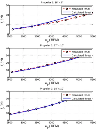
Three different sizes of propellers4, 16"×8", 17"×10" and 18"×10", are used in this ex-periment to generate thrust at different rotational speeds. The same propellers are consid-ered in Eq. (3.7) to calculate the predicted thrust for the same range of rotational speeds used in experiment. Figure 3.3 plots the measured thrust and the calculated thrust for each propeller vs. the rotational speed of the propeller.

4_{Each propeller is denoted by: diameter×pitch length. Theinch(") is used to be the measurement}

25000 3000 3500 4000 4500 5000 5500 10

20 30

Propeller 1: 16" × 8"

f p

(

N)

ω

p ( RPM)

measured thrust Calculated thrust

25000 3000 3500 4000 4500 5000 5500

10 20 30 40

Propeller 2: 17" × 10"

f p

(

N)

ω

p ( RPM)

measured thrust Calculated thrust

25000 3000 3500 4000 4500 5000 5500

10 20 30 40

Propeller 3: 18" × 10"

f p

(

N)

ω

p ( RPM)

measured thrust Calculated thrust

Figure 3.3: Measured thrust and calculated thrust vs. rotating speed for three different propellers.

and it is only 1.52% in the largest propeller (18"×10") for the plotted range of the rotation speed. Moreover, the derived model overestaimes the real generated thrust for the smallest propeller while it underestimates the generated thurst for the other two propellers.

The result of this experiment can be interpreted in light of the simplification of the mo-mentum theory and the assumptions made while deriving the thrust formula. The assump-tion of uniform inflow seems to be reasonable for large blade propellers. As the diameter of the propeller decreases, the inflow becomes disturbed and not uniform any more. The impact of the blade size increases proportional to the rotational speed of the propeller, and in this case the assumption of a uniform flow becomes questionable.

In conclusion, we can say that for the purpose of propulsion systems design, Eq. (3.7) represents a good approximation for the thrust model of air propellers within specific range of radius and pitch sizes. For propellers outside this range, a safety margin needs to be considered to compensate for the inaccuracy of the derived thrust model. If a more accurate model is sought for the thrust, it can be obtained by using the element blade theory or any other alternative in hand. It can follow also that the power model in Eq. (3.11) has a similar accuracy to that obtained in the thrust model. However, the power model is of higher order in terms of the rotation speedωp, which puts more limitation to

the accuracy of power model for high rotational speed and small propellers.

3.2.3

Electric Motors

types of electric motors available commercially that can be used for the electric propul-sion system. Recently, brushless DC (BLDC) motors have gained enormous popularity in UAV applications due to the high torque-to-weight ratio, high efficiency, low noise level, high reliability and long lifetime of these motors [58]. In general, BLDC motors are more expensive than conventional DC motors with brushes, yet, they are much more efficient [59]. BLDC motors exist in a wide range of sizes, weights, power ratings, and they fit into many applications. The operating principle of brushless DC motor is based on electric commutation instead of mechanical commutation that exists in DC motor with brushes. In the sequel, we consider BLDC motors as the standard motors for the propul-sion system design. However, the design method and motor’s modeling remain valid for other types of DC motors.

Assuming negligible mechanical and electrical losses, the electric input powerP_in to the BLDC motor and the output mechanical powerP_outat the shaft can be written respectively asPin=VinIin andPout=ωmτm, whereVinandIinare the supplied DC voltage and current from the battery pack respectively. τm is the torque developed at the shaft of the motor andωmis the rotational speed of the shaft. The relation between the input and out power is given by:

P_out

P_in =

τm

I_in ·

ωm

V_in =kikv, (3.15)

wherekvandkiare known respectively as the rotational speed-to-voltage constant and the torque-to-current constant (also known as the voltage and the torque constants). These two constants of electric motors are used to determine the electric power needed to load a certain propeller at a specified rotational speed. Mathematically, we write:

Vin =

ωm

k_v , Iin=

Pout

ωmki

. (3.16)

Assuming a direct driving of the propeller, we can write:

V_in =ωp

k_v , Iin=

P_fp

ωpki

. (3.17)

whereωpandPfp are as defined in the previous section.

supplied to the motor wherek_v is given as a constant for the motor. Likewise, the current needed to produce a mechanical powerP_fp necessary to rotate the propeller at speedωp depends onki. In practice,kv is given by the technical specifications of the motor while

kiis rarely supplied in motor specifications. This is due to the fact thatkiis not constant at all operating points and rather it is a function of many factors such as the ratio between output power and the rating power of the motor and the temperature of the motor [60]. Instead, manufacturers supply operational curves and load charts of the motor that can be used to obtain the mapping between the supplied voltage to the motor and the expected drawn current under the load of different propellers. Figure 3.4 shows an example of the load curves for the BLDC motor (HC6332-230) manufactured by "Maxx product"5.

The HC6332-230 motor has an efficient current rating range of 30−80 A. The graph shows the drawn current vs. the supplied voltage for different propellers. For instance, the motor draws approximately 44Awhen loaded with the propeller 15"×10" and supplied by 40V. Propellers that are not shown in the graph can be fitted in by approximate matching with the propellers presented in the graph. For instance, empirical experiments show that within a specific range of sizes, adding two inches to pitch equals to decreasing one inch in diameter; i.e., keeping the voltage level fixed, this motor draws approximately the same current under the load of 19"×10" or 18"×12" [61].

3.2.4

Electric Speed Controllers (ESCs)

ESCs are used to control the speed of electric motors and therefore the speed of the pro-pellers to generate the required thrust. ESCs are electronic circuitries that receive refer-ence signals from the user and accordingly regulate the voltage from the power supply to control the rotational speed of the controlled motors. The current and voltage rate of the ESC should match with the current rating and the operating voltage of the motor. In case of a BLDC motor, the ESC runs the appropriate electric switching sequence necessary to control the supply voltage and operate the motor. Moreover, a BLDC motor needs a des-ignated ESC for brushless motors and cannot be controlled by other types of ESC. In the proposed design procedure, it is assumed that negligible power loss occurs at the ESC. In addition, the size and weight of the ESC are negligible compared to other principle components of the propulsion system. Therefore, the ESC is not an important component to be considered in the proposed design procedure.

3.2.5

Battery Packs

the maximum drawn current is high and vice versa). The operating time of the chosen battery pack, and hence the flight time of the vehicle, depends on the drawn current and the current rating of the battery pack. Mathematically, the battery pack is represented by:

V_b=V_b0−I_bR_b , I_bmax =c_bmaxI_b0 , t_b= Ib0(A.h)

I_b(A) , (3.18)

whereV_bis the effective voltage at the terminal of the battery,V_b0 is the nominal no-load voltage rate,I_bis the drawn current from the battery andR_bis the internal resistance of the battery pack. The maximum current that can be drawn from the battery isI_bmax whileI_b0

is the current rate of the battery and is defined as the current that can be supplied from the battery for one hour before the rated voltage starts to drop, i.e. it is given in Amber-hour (A.h). c_bmax is the maximum discharging rate of the battery and is defined by the battery manufacturer. t_bis the operating time of the battery before the voltage drops beyond the nominal value. The unit oft_b is (hours). This due to the fact that the current rate of the batteryI_b0 is given in (A.h) and the required current for the propeller is given in (A).

3.3

Design Methodology

This section proposes a systematic procedure for designing the propulsion system of elec-trically driven VTOL rotary-wing UAV, assuming that the total size of the vehicle, includ-ing propellers’ dimension, is specified. In addition, the maximum permissible weight of the vehicle including the propulsion system and the maximum payload is estimated a priori. The minimum continuous flight time needs to be specified as well.

The estimated size and structure of the UAV puts a radius restriction R_max on selecting the size range of propellers that can be used for the propulsion system design; i.e.,R_p≤

practical aspects of the design puts limits on the size of propellers that can be used in the design procedure.

The total weight of the UAV system includes the weight of the mechanical structure, on-board equipment, the propulsion system and payload. Given the estimated total weight of the vehicle M_total, the design objective of the propulsion system is always to achieve a taking-off thrust f_h >M_total using the lightest possible components available in the market. The weight of the ESC and the propeller are negligible compared to the weight of the battery pack and electric motor which contributes the major part of the propulsion system’s weight.

The propulsion system should enable the UAV to fly at least for a specified flight time

t_fmin. The minimum flight time is important to decide on the required battery pack that in turn affects the weight of the propulsion system. Hence, a good propulsion system design calls for maximum thrust-to-weight ratio while achieving maximum possible flight time.

In total, the inputs to the design procedure are (i) the maximum allowable radius of the propeller:R_max, (ii) the total weight of the UAV:M_total, (iii) the allowance for the propul-sion system weight: M_smax =M_total−M_pl whereM_pl is known and it is the weight of the vehicle structure6and desired payload, and (iv) the required minimum flight time,t_fmin.

Design Procedure

Given the design specifications ofM_total,M_smax andt_fmin, the following steps are proposed to design the electric propulsion system for VTOL UAVs:

1. Set the required thrust f_h=αMtotal, whereα >1 is a safety factor to be chosen by the designer (e.g.α ≈1.2).

2. Selecting a set of propellers:

6_{The structure weight includes all components for control, signal processing and other on-board}

(a) Choose a set of commercially available propellers _P whose radius are R_p≤

R_max∀ p∈_P. The set_Pmay contain propellers of same radius but different pitches. If the pitch of the propeller is specified in terms of pitch lengthβp,

obtain its pitch angleθpusing Eq. (3.14).

(b) For each propeller p ∈ _P, calculate the minimum rotational speedωp (using Eq. (3.6) and Eq. (3.8)) and the corresponding minimum mechanical power

P_fp (using Eq. (3.11) or Eq. (3.12)) necessary to generate t