Comparative analysis of machine learning algorithms for computer-assisted reporting based on fully automated cross-lingual RadLex® mappings
Máté E. Maros 1,2,*, MD, MSc; Chang Gyu Cho1,2; Andreas G. Junge1, BSc; Benedikt
Kämpgen3, PhD; Victor Saase1 MD, MSc, Fabian Siegel2 MD, Frederik Trinkmann2 MD,
Thomas Ganslandt2, PhD, MD; Holger Wenz1, MD
1Department of Neuroradiology, Medical Faculty Mannheim, Heidelberg University,
Mannheim, Germany.
2Department of Biomedical Informatics at the Heinrich-Lanz-Center, Medical Faculty
Mannheim, Heidelberg University, Mannheim, Germany.
3Empolis Information Management GmbH, Kaiserslautern, Germany.
*Correspondence to:
Máté E. Maros, MD, MSc
Department of Neuroradiology,
Medical Faculty Mannheim, Heidelberg University, Mannheim, Germany
Theodor-Kutzer-Ufer 1-3,
68137 Mannheim, Germany
Tel: +49-621-383-2443, Fax: +49-621-383-2165,
E-mail: [email protected]
ORCID iD: 0000-0002-1589-8699
Keywords: machine learning, computer-assisted reporting (CAR), RadLex®, natural language
processing (NLP), contextual reporting, The Alberta Stroke Programme Early CT Score
(ASPECTS).
Tables: 3; Figures: 4.
Word count: 3951
Highlights
• Cross-lingual RadLex® mapping-based machine learning can improve radiological
report quality by context-sensitively suggesting key imaging biomarkers.
• Human expert-based key information extraction and fully automated RadLex®-based
machine learning are comparable.
• By increasing key information content in reports, embedded assistive algorithms can
substantially improve cohort selection for downstream analytics.
• The presented approach is robust and requires only a limited amount of expert labeled
training data even for imbalanced classification tasks.
• We open-source our framework to facilitate research on developing task specific
Abstract
Objectives: Studies evaluating machine learning (ML) algorithms on cross-lingual RadLex® mappings for developing context-sensitive radiological reporting tools are lacking. Therefore, we investigated whether ML-based approaches can be utilized to assist radiologists in providing key imaging biomarkers – such as The Alberta stroke programme early CT score (APECTS).
Material and methods: A stratified random sample (age, gender, year) of CT reports (n=206) with suspected ischemic stroke was generated out of 3997 reports signed off between 2015-2019. Three independent, blinded readers assessed these reports and manually annotated clinico-radiologically relevant key features. The primary outcome was whether ASPECTS should have been provided (yes/no: 154/52). For all reports, both the findings and impressions underwent cross-lingual (German to English) RadLex®-mappings using natural language processing. Well-established ML-algorithms including classification trees, random forests, elastic net, support vector machines (SVMs) and boosted trees were evaluated in a 5 x 5-fold nested cross-validation framework. Further, a linear classifier (fastText) was directly fitted on the German reports. Ensemble learning was used to provide robust importance rankings of these ML-algorithms. Performance was evaluated using derivates of the confusion matrix and metrics of calibration including AUC, brier score and log loss as well as visually by calibration plots.
Results: On this imbalanced classification task SVMs showed the highest accuracies both on human-extracted- (87%) and fully automated RadLex® features (findings: 82.5%; impressions: 85.4%). FastText without pre-trained language model showed the highest accuracy (89.3%) and AUC (92%) on the impressions. Ensemble learner revealed that boosted trees, fastText and SVMs are the most important ML-classifiers. Boosted trees fitted on the findings showed the best overall calibration curve.
Graphical abstract
Embedded Computer-Assisted Reporting (CAR)
● ● ● ● ● ● ● ● ● ● ● ● ● ● ● ● ELNET−impr−p675−1 fasttext−find−yes fasttext−impr−yes SVM−e1071−find−p907−yes SVM−e1071−impr−p675−yes tRF−BS−impr−p675−yes tRF−LL−impr−p675−yes vRF−impr−p675−p200−yes XGBOOST−find−p907−yes XGBOOST−impr−p675−yes 2 4 6
0.00 0.01 0.02
accuracy_decrease g in i_ d e c re a se p_value ● ● ● ● <0.01 [0.01, 0.05) [0.05, 0.1) >=0.1 variable top
Multi−way importance plot
● ● ● ● ● ● ● ● ● ● ● ● ● ● ● ● ELNET−impr−p675−1 fasttext−find−yes fasttext−impr−yes SVM−e1071−find−p907−yes SVM−e1071−impr−p675−yes tRF−BS−impr−p675−yes tRF−LL−impr−p675−yes vRF−impr−p675−p200−yes XGBOOST−find−p907−yes XGBOOST−impr−p675−yes 2 4 6
0.00 0.01 0.02
accuracy_decrease g in i_ d e c re a s e p_value ● ● ● ● <0.01 [0.01, 0.05) [0.05, 0.1) >=0.1 variable top
Multi−way importance plot
Classifier importance plot
0.00 0.25 0.50 0.75 1.00
0.00 0.25 0.50 0.75 1.00
Mean prediction O b s e rv e d f ra c ti o n Method SVM−LK findings SVM−LK impressions
Reliability Plot − Tumor diagnosis: yes
0.00 0.25 0.50 0.75 1.00
0.00 0.25 0.50 0.75 1.00
Mean prediction O b s e rv e d f ra c ti o n Method fastText findings fastText impressions
Reliability Plot − Tumor diagnosis: yes
0.00 0.25 0.50 0.75 1.00
0.00 0.25 0.50 0.75 1.00
Mean prediction O b s e rv e d f ra c ti o n Method
Ensemble vRF predicted probabilities
Reliability Plot − Tumor diagnosis: yes
0 5 10 15 20 25
0.00 0.25 0.50 0.75 1.00
Ensemble vRF predicted probabilities
0.00 0.25 0.50 0.75 1.00
0.00 0.25 0.50 0.75 1.00
Mean prediction O b s e rv e d f ra c ti o n Method XGBoost findings XGBoost impressions
Reliability Plot − Tumor diagnosis: yes
Calibration plots
outer fold 2.0
Outer fold 1.0
TRAINING SET
Human Expert Annotated
Features (HEAF)
Findings
Cross-lingual NLP-based fully automated
RadLex® mapping
Reports
Im-pressions
5 x 5-fold nested cross validation
N = 206
Ntraining 1.0= 164
TEST SET
Ntest 1.0= 42
N e st ed C V 1.5 34 1.1 32 .. . ... ...
Ntraining 5.0= 166
... ... ...
...
..
.
...
Random Forests (RF)
Support Vector Machines (SVM) Boosted Trees (XGBoost) Elastic Net (ELNET) FastText*
34 33 33 32 32
�Ntest 1.1-1.5 =Ntraining 1.0= 164
�
Outer fold 5.0
Machine Learning Classifier
Train
Train
Train
Ensemble models
RF & XGBoost
Predict � Im p o rt a n c e R an ki n g .. .
Ntest 5.0= 40
... Predict P re d ic t ... ... ... ASPECTS recommended:
yes (154) vs. no (52)
Ntraining 1.5= 132
1. Introduction
There are no studies available that evaluate machine learning (ML) algorithms on cross-lingual RadLex® mappings to provide guidance when developing context-sensitive radiological reporting tools. Therefore, the purpose of our study was to compare the performance of ML algorithms developed on features extracted by human experts against those developed on fully automated cross-lingual RadLex® mappings of German radiological reports to English[1], in order to assist radiologists in providing key imaging biomarkers such as The Alberta Stroke Programme Early CT Score (APECTS)[2]. We show that this fully automated RadLex®-based approach is highly accurate even if the ML models were trained on limited and imbalanced expert labelled data sets[3-6]. Hence, this work provides a valuable blueprint for developing ML-based embedded applications for context-sensitive computer-assisted reporting (CAR) tools[7-10].
RadLex® is a comprehensive hierarchical lexicon of radiology terms that can be utilized in reporting, decision support and data mining[3]. RadLex® is freely available (v.4.0, http://radlex.org/) from the Radiological Society of North America (RSNA). It provides the foundation for further ontologies and procedural data bases such as the LOINC/RSNA Radiology Playbook[11] or Common Data Elements (CDE; RadElement; https://www.radelement.org/)[12]. The official translation of RadLex® to German by the German Society of Radiology (DRG) was made public in January 2018 and contained over 45,000 concepts.
development using their data[18, 19]. Nonetheless, these key predictors are frequently missing from radiological reports as their overwhelming majority is still created as conventional narrative “free-text”[1, 20, 21].
ML methods have been introduced as powerful computer-aided diagnostic (CAD) tools[9, 15, 22] not only in image recognition and classification, but also in radiological reporting[23, 24]. Recently, complex deep transformer-based language models (TLM) are becoming the state-of-the-art (SOTA) in natural language processing (NLP)[25-29]. However, these models need considerable amount of general and domain specific corpora for training (even if using transfer learning approaches), which are scarce for languages other than English, particularly in the medical domain where creating expert-labelled high-quality training data is extremely resource intensive[30-33]. Despite achieving SOTA on certain classification tasks, TLMs represent black box methods and show susceptibility to subtle perturbances[31, 32]. Additionally, TLMs are seldom compared to baseline information retrieval methods such as shallow ML algorithms or linear classifiers (fastText) developed on bag-of-words (BOW)[34-36]. Therefore, we performed comprehensive analyses using an ensemble learning framework (Figure 1) that combined well-established ML algorithms as base classifiers including random forests (RF)[37], regularized logistic regression (ELNET)[38, 39], support vector machines (SVM)[40] and classification- (CART)[41] and boosted trees (XGBoost)[42] as well as fastText[36] on German computed tomography (CT) reports with suspected stroke and on their cross-lingual English RadLex® mappings using NLP[43].
2. Materials and methods
2.1 Study cohort
The study was approved by the local ethics committee (approval nr.: 2017-825R-MA). Written
informed consents were waived by the ethics committee due to the retrospective nature of the
analyses. In this single-center retrospective cohort study, consecutive (German) radiological
reports of cranial CTs with suspected ischemic stroke or hemorrhage between 01/2015-12/2019
were retrieved from local RIS (Syngo, Siemens, Healthineers, Erlangen, Germany) that
contained the following key words in the clinical <request reason>, <request comment> or
<request technical note> fields: “stroke”, “time window for thrombolysis”, “wake up”,
“ischemia” and their (mis)spelling variations. A total of 4022 reports fulfilled the above criteria.
After data cleaning, which excluded cases with missing requesting department, 3997 reports
remained. Next, we generated a stratified random subsample (n=207, ~5.2%) based on age
(binned into blocks of 10 years), sex (M|F), year (in which the imaging procedure was
performed) and requesting department. During downstream analyses one report was removed
because it contained only a reference to another procedure, leaving n=206 for later analyses
(Figure 1). The extracted reports were all conventional free-texts and were signed off by senior
radiologists with at least 4 years of experience in neuroradiology.
2.2 Information extraction by human experts
Three independent readers (R1, experience 3yrs; R2, 7yrs; R3, 10yrs) assessed the clinical
questions, referring departments, findings and impressions of the reports. For each report, all
readers independently evaluated whether ASPECTS was provided in the report or should have
been provided in the report text (necessary: 154, 74.7%; not meaningful: 52, 25.3%]). Further,
the two senior experts (R2 and R3) manually extracted clinico-radiologically relevant key
features in the context of whether reporting ASPECTS is sensible based on the presence (yes
bleeding (separately for each of the following entities: intracerebral hemorrhage (ICH), epi-
(EDH), subdural hematoma (SDH), subarachnoid hemorrhage (SAH)); tumor; procedures
including CT-angiography (CTA) or CT-perfusion (CTP); whether cerebral aneurysms or
arteriovenous malformations (AVM) were detected; previous neurosurgical (clipping, tumor
resection) or neurointerventional procedures (coiling); and previous imaging (within the last
1-3 days)[44, 45]. These human expert-annotated features (HEAF) were extracted concurrently
from both the finding and impression sections and selected in accordance with national and
international guidelines for diagnosing acute cerebrovascular diseases[44, 45]. HEAFs were
used as input for ML algorithm development (Table 1). The feature matrix is available as
supplementary data (heaf.csv) or GitHub download
(https://github.com/mematt/ml4RadLexCAD/data).
2.3 RadLex® mapping pipeline
Both the findings and impression sections of each German report (n=206) were mapped to
English RadLex® terms using a proprietary NLP tool, the Healthcare Analytics Services®
(HAS) by Empolis Information Management GmbH (Kaiserslautern, Germany;
https://www.empolis.com/en/). HAS implements a common NLP pipeline consisting of
cleansing (e.g., replacement of abbreviations), contextualization (e.g. into segments "clinical
information", "findings", and "conclusion"), concept recognition using RadLex®, and negation
detection ("affirmed", "negated", and "speculated")[46]. For concept recognition, a full text
index and morpho-syntactic operations such as tokenization, lemmatization, part of speech
tagging, decompounding, noun phrase extraction and sentence detection were used. The full
text index is an own implementation with features such as word/phrase search, spell check and
ranking via similarity measures such as Levenshtein distance and BM25[47, 48]. The index is
populated with synonyms for all RadLex® entities (both from the lexicon and by manual
Basis Technology® (Cambridge, MA, USA;
https://www.basistech.com/text-analytics/rosette/). For accuracy, RBL uses machine learning techniques such as perceptrons,
support vector machines, and word embeddings. For negation detection, the NegEx algorithm
was implemented in UIMA RUTA[46, 49]. No further pre-processing steps of the text were
done.
Our RadLex® annotation and scoring pipeline (RASP), which utilizes the aforementioned API
by Empolis, is available as a Shiny application at mmatt.shinyapps.io/rasp [35]. We used RASP
to generate the document (i.e. report RadLex®) term matrix (DTM) of the complete data set
over all reports (n=206) both for the findings and impression sections, respectively. In the DTM,
each report is represented as a vector (i.e. bag-of-)RadLex® terms that occurred in the
corpus[34, 35]. RadLex® terms were encoded in a binary fashion (0|1), whether the term was
present or not. Further, each RadLex® term (i.e. feature) was annotated with three levels of
confirmation or confidence “affirmed”, “speculated”, “negated”, which was included in the
feature name. This DTM provided the basis for fully automated RadLex®-based ML algorithm
development (Table 2). The report-RadLex® term-matrices (i.e. DTMs) both for the findings
and impression sections are available for direct download from our GitHub repository
(https://github.com/mematt/ml4RadLexCAD/data) or as supplementary data
(radlex-dtm-findings.csv and radlex-dtm-impressions.csv).
The performances of ML algorithms developed on these automated NLP-RadLex® mappings
were then compared to those ML algorithms that were developed on the features extracted by
human experts (HEAF). It is of note, however, that in its current iteration (v4.0) RadLex® does
not contain certain key terms or concepts, one of which is ASPECTS. Although there is a CDE
for ASPECTS classification (https://www.radelement.org/element/RDE173)[12]. Hence,
extended IDs had to be created for such terms in the NLP annotation service, which are denoted
2.4 Machine learning setup and classifier development
We performed extensive comparative analyses of well-established ML algorithms (base
classifiers) to automatically learn rules required for ASPECTS reporting including single
classification (and regression) trees (CART)[41], random forests (RF)[37], boosted decision
trees (XGBoost)[42], elastic net-penalized binomial regression (ELNET)[38, 39] and support
vector machines (SVM)[40]. Single CART was used to represent the baseline ML algorithm.
A CART has the advantage that human readers can more easily interpret it, however its
estimates are much less robust than ensembles of trees like RF[41, 50-52].
Each ML algorithm was fitted to the i) human expert-annotated features (HEAF; Table 1) and
to the ii) RadLex® mapped DTMs both for the findings and impressions separately (Table 2).
Because the effort of manually annotating the data set is large, especially if multiple experts
annotate the same reports, we built upon our previously open-sourced protocol of a 5-fold
nested cross-validation (CV) resampling scheme to have an objective and robust metric when
comparing the performance of the investigated methods (Figure 1). Nested CV schemes allow
for the proper training of secondary (e.g. calibrator or ensemble) models, without allowing for
information leakage (Figure 1). To counter act the class imbalance (yes:no = 3:1) during
CV-fold assignment (nCV-folds.RData), we performed stratified sampling. Also, RFs were
downsampled to the minority class during training [53, 54].
In brief, the data set (n=206) was divided into stratified subsamples (outer fold training
[nouter.train=~164-166] – test set pairs [nouter.test=40-42]) using 5-fold cross-validation (Figure 1;
dashed blue and red boxes). Then, only the outer fold training sets were, yet again, subsampled
using 5-fold CV, in order to create the nested/inner fold (training [ninner.train=130-134] – test set
pairs [ninner.test=32-34]; Figure 1, nested CV). This was performed for both the findings and
impressions sections using identical fold structures (Figure 1).
Hyperparameter tuning (i.e. training) of the investigated ML algorithms (base classifier) was
were fitted to the same data structure. Also, random seeds were fixed across all ML algorithms,
in order to ensure direct comparability of their performance measures. ML algorithm training
was optimized using either accuracy, brier score or log loss, which is indicated along the tuning
parameter settings in Tables 2 & 3. For all ML algorithms probability outputs were also
recorded and used to measure AUC and to create calibration plots. The average 5-fold CV
model performances on the outer fold test sets are provided in Tables 1, 2 & 3.
Furthermore, we investigated whether a second layer ensemble model (based on all evaluated
ML-base classifiers) could improve the overall performance. This second layer algorithm
(either RF or XGBoost) was trained on the combined predictions (i.e. “ensemble”) of the base
ML models (i.e. CART, RF, XGBoost, ELNET, SVM and fastText) on the respective
nested/innerfold test sets (Figure 1). Then, this tuned model was evaluated on the corresponding
outer fold test set preventing any information leakage[6]. Additionally, the second layer
“meta/ensemble” learner was used to derive importance rankings of the investigated ML base
classifiers. For this, we have used mean decrease in accuracy without scaling when RF was
used as the second layer “meta/ensemble” model, which has been suggested as the most robust
setting when testing correlated features[6, 53, 55, 56]. Variable importance plots describing the
RF meta-learner (Figure 3) were created using the randomForestExplainer package
(v0.10.0.)[57]. Similarly, for importance ranking of boosted decision trees the gain metric was
used[42]. Heretofore, we refer to second layer RF and XGBoost algorithms as meta/ensemble
learners or models.
2.5 Text classification directly on German report texts using fastText
We used the open-source, lightweight fastText library (v0.9.1; https://fasttext.cc/) to learn linear
text classifiers for ASPECTS recommendations on our data set[36] . The German report texts
(both findings and impression sections) were preprocessed by excluding “([-.!?,'/()])”. It is of
subset of ~130-165 reports and we did not utilize any pre-trained word vector model for
German[58]. This approach ensured a more direct comparability with the ML-classifiers
developed on bag-of-RadLex® mappings. However, pre-trained word vector models for 157
languages, which were pre-trained on Common Crawl and Wikipedia by the fastText package
authors are available for direct download (https://fasttext.cc/docs/en/crawl-vectors.html) [58].
We used the Python (v3.7) interface to fastText
(https://github.com/facebookresearch/fastText/tree/master/python) on an Ubuntu 19.10
machine. FastText models were fitted both on the findings and impression sections respectively,
using the same 5 x 5-fold nested-CV scheme as for the other ML algorithms with similar
extra-nested CV loop for training on the outer- or inner fold training sets. Class label predictions and
probability outputs were recorded and evaluated in the same manner as the investigated ML
algorithms developed on HEAF and RadLex® mappings.
2.6 Statistical analyses
All statistical analyses were performed using the R language and environment for statistical
programming (R v3.6.2, R Core Team 2019, Vienna Austria). The Cohen’s kappa statistic was
used to assess inter-rater agreement whether ASPECTS is recommended in a pairwise fashion
for each of the two readers. To assess the overall agreement among the three readers, Fleiss’
and Light’s kappa was used.
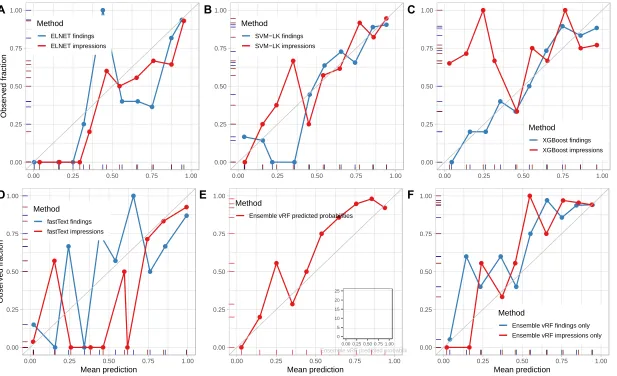
Additionally, we created custom functions
(https://github.com/mematt/ml4RadLexCAD/tree/master/calibration plots) to visualize the
probability outputs (i.e. calibration profiles) of the investigated ML-classifiers (Figure 3). Such
calibration plots (or reliability diagrams) are useful graphical tools to visually assess the quality
of calibration[59, 60]. Briefly, for real-life problems the true conditional probabilities are
unknown, therefore the prediction space needs to be discretized into bins [60, 61]. A common
probabilities fall. For each bin the fraction of true positive cases (y-axis) is plotted against the
mean of predicted classifier values (x-axis). Hence, an ideally calibrated classifier would lie on
3. Results
3.1 Inter-rater reliability of human experts
Providing ASPECTS in the report would have been recommended by R1 in 156 (75.7%), by
R2 in 154 (74.8%) and by R3 in 155/206 (75.2%) of the cases. The overall agreement between
the three readers for “ASPECTS recommended” was kappaLight=0.747 (n=206, z=4.6,
p=4.3×10⁻⁶). The pairwise Cohen’s kappa between R1 and R2 was 0.635 (p<2×10-16), which
corresponded to 86.4% agreement. Between R1 and R3 it was 0.62 (p<2×10-16) corresponding
to 85.9% agreement. Ratings of two (R2 and R3) experienced readers showed an almost perfect
alignment kappa=0.987 (p<2×10-16) with 99.5% overall agreement.
3.2 Reliability between automated RadLex® mappings and expert-annotated labels
In this random subsample, which represents a robust cross-section of the daily praxis,
ASPECTS was reported extremely rarely in 4/206 (1.9%). Three of which occurred both in the
findings and impressions (3/4, 75%) section and one of which was only reported in the
impression (1/4, 25%). The RASP tool correctly annotated all ASPECTS-negative (203/203)
and ASPECTS-positive (3/3) finding sections. In the impressions, it misclassified one
ASPECTS-positive (1/4, 25%) report as negative (1/206, 0.49%).
3.3 Performance of machine learning algorithms developed on human expert-annotated
features (HEAF)
3.3.1 Single classification tree (CART)
CART demonstrated a 5-fold CV accuracy of 73.3% with the worst 63% AUC, BS (0.37) and
LL (0.87) values among the tested ML-classifiers (Table 1).
The default (“vanilla”) RF classifier fitted on the 28 HEAF achieved a 5-fold CV accuracy of
81.5% with an AUC of 82% and corresponding BS and LL of 0.27 and 0.44, respectively (Table
1). Drastically reducing the feature space of vRF to only the nine (9/28: 32.1%) or five (5/28;
17.9%) most important predictors, had a comparably limited effect on the predictive
performance of vRF: its accuracies decreased 12.8% and 7.7%, respectively; AUC decreased
by ~16%; while BS (~37%) and LL (~27%) scores increased (Table 1).
Fine tuning the RF classifier using the BS (tRFBS)and LL (tRFLL)metrics slightly improved the
overall accuracy without relevantly changing the calibration metrics of the vRF algorithm
(Table 1). On the outer folds, both tRFBS and tRFLL limited the feature space similarly – to the
14 or 25-28 most important variables. Interestingly, ME-optimized RF (tRFME) achieved a
slightly worse overall performance profile. Notably, on the outer fold 4.0, it limited the feature
space to only the five RadLex® terms.
3.3.3 Elastic net-penalized binomial regression (ELNET)
ELNET showed a similar performance profile to RFs when fitted on the 28 HEAF but it
achieved a narrower 5-fold CV confidence range of its accuracies (78-86%) while obtaining
similar AUC, BS and LL scores (Table 1). The mixing parameter alpha (𝛼) was chosen 3 out
of 5 times to fit ridge (0) or ridge-like (0.1, 0.1) models while twice to fit lasso (1) or lasso-like
(0.8) models on the outer folds.
3.3.4 Support vector machines (SVM)
On HEAF linear kernel SVMs (SVM-LK) achieved the highest 5-fold CV accuracy (87.4%)
and lowest BS (0.22) and LL (0.37) scores while obtaining a similar AUC of ~80% to other ML
classifiers (Table 1). The tuning parameter of C was selected as 1 on two outer folds suggesting
a larger margin for the separating hyperplane while larger values of 10 or 100 were selected on
3.3.5 Boosted decision trees (XGBoost)
Boosted decision trees were similarly accurate (80.6%) like tuned RF and ELNET. Despite the
detailed tuning grid, XGBoost had overall somewhat worse performance profile than the other
investigated ML algorithms, particularly AUC was lower at 70% for which we do not have a
clear explanation.
3.4 Performance of machine learning algorithms developed on fully automated RadLex®
mappings
3.4.1 Single classification tree (CART)
Directly applying a classification tree without optimizing its tree complexity (i.e. no pruning)
showed on the findings similar overall accuracy (77.2%) to vRF with similar AUC and BS
(Table 2) but with worse LL metrics. On the impressions, however, CART was tied for the 3rd
best accuracy (85.0%) but still it showed low AUC (0.75) and high LL (0.58) values.
3.4.2 Random forests (RF)
Applying unsupervised variance filtering to select the top 33% most variable RadLex®
mappings of the findings sections, improved the 5-fold CV accuracy of vRF by ~4.7%. In
contrast, the same variance filtering on the impression sections did not relevantly (0.6%)
improve vRF’s accuracy (Table 2). Tuned RF models were slightly more accurate than the
default vRF, however, tuning did not improve much upon the remaining calibration metrics.
3.4.3 Elastic net-penalized binomial regression (ELNET)
ELNET was the 3rd best-performing ML algorithm on the RadLex® features of the findings
sections behind SVMs and XGBoost with similar BS and LL metrics but lower accuracy
5-fold CV accuracy (85.0%; 95%CI: 79.3-89.5%; pAcc.vs.NIR = 2.8×10⁻⁴) with corresponding
second-best calibration profile (AUC: 86%; BS: 0.22; and LL: 037). On the outer folds of the
impressions lasso or lasso-like settings (0.9-1) dominated the tuned 𝛼 settings. ELNET had a
better visual calibration profile on the impressions than on the findings (Figure 2A).
3.4.4 Support vector machines (SVM)
Linear kernel SVMs (SVM-LK) were the only classifiers that performed in the top 2 on the
RadLex® feature spaces of both the findings (pAcc.vs.NIR = 5.1×10⁻³) and impressions (pAcc.vs.NIR
= 1.4×10⁻⁴) sections (Table 2). SVM-LK had the highest AUC and lowest LL on the findings
while on the impressions, it was overall the best-performing base ML-classifier. SVMs were
comparably well-calibrated for both the findings and impressions, especially in the 0.5-1.0
probability domain (Figure 2B).
3.4.5 Boosted decision trees (XGBoost)
XGBoost performed particularly well on the RadLex® mappings of the findings – where the
other ML algorithms (including fastText) struggled (Table 2). It showed the highest accuracy
(pAcc.vs.NIR = 1.4×10⁻⁴) and lowest BS with corresponding slightly worse AUC and LL metrics
(than the runner-up SVM-LK). Nevertheless, it had the best overall visual calibration profile on
the reliability diagrams for the whole probability domain (Figure 2C). Compared to the
findings, on the impressions XGBoost tuning implied a stronger subsampling of the features
when constructing each tree, thereby strongly limiting the available predictor space. On the
impressions, XGBoost performed similar to RF classifiers.
3.5. Linear models (fastText) fitted directly on German report text
When directly fitting the findings sections of the reports, the fastText algorithm showed a
and specificity of 48.1% (PPV 84.4%, NPV: 75.8%), which corresponded to 84.4% precision
and 89.3% F1 score. It achieved comparable AUC (81.1%) and BS (0.29) to other shallow
ML-models trained on RadLex® mappings but showed markedly worse LL profile (0.98)
suggesting “more certain” misclassifications.
FastText achieved the best results across all investigated ML algorithms fitted on the
impressions sections of the reports. It showed a 5-fold CV accuracy of 89.3 % (95%CI:
84.3-93.2%; pAcc.vs.NIR = 1.35× 10⁻⁷) with a balanced accuracy of 82.0%. Its predictive profile was
in the 87-97% range (sensitivity: 96.8%; specificity: 67.3%; PPV 89.8%, NPV: 87.5%) with
precision of 89.8% and F1 score of 93.1%. Furthermore, it showed the highest AUC (91.7%)
with lowest BS (0.18) but yet again somewhat worse LL (0.55) than the RadLex®-based ML
algorithms. FastText showed poor visual calibration profiles for both the findings and
impressions in the lower probability domains (0-0.5), however it was almost ideally calibrated
in the 0.75-1.0 domain of the impressions (Figure 2D).
3.6 Performance of the second layer meta/ensemble-learners
The second layer meta/ensemble RF learner, which was trained on predictions of the
ML-classifiers of the findings sections, showed similar performance metrics (Table 3) as the top
single ML-classifiers like SVM-LK, fastText and XGBoost (Table 2). Its accuracy was in the
77-88% 95%CI range (pAcc.vs.NIR = 1.8 ×10⁻⁴) with 89.6% sensitivity; 65.3% specificity; 88.5%
PPV; and 68% NPV which corresponded to a precision of 88.5% and F1 score of 89.6%.
SVM-LK was chosen twice as the most important classifier while vRF, ELNET and XGBoost were
each selected once on the five other folds (Figure 3A & D).
The 5-fold CV accuracy (89.3%) of the ensemble RF (Table 3), when using only the
ML-models of the impressions as input features, was identical to the best predictor (fastText). But
the 95% confidence interval got narrower and the LL score got considerably reduced (by 38%).
specificity 80.8%; PPV 93.4%, NPV 77.8% with corresponding precision of 93.4% and F1
score of 92.8%. FastText was chosen as the most important predictor for all outer fold test sets
while as top 2nd predictor XGBoost was chosen twice; ELNET, SVM-LK and tRFBS were each
selected once, respectively (Table 3; Figure 3B & E).
When the ML-classifier predictions of both the findings and impressions were the combined
input for the second layer RF model, its accuracy, BS and LL slightly got worse (5-6%). The
confusion matrix derivates were as follows: sensitivity 91.6%; specificity 80.8%; PPV 93.4%,
NPV 76.4% with corresponding precision of 93.4% and F1 score of 92.5%. The variable
importance rankings were dominated by ML-classifiers developed on the impression sections
(Table 3; Figure 3C & F). The visual calibration profile of the RF ensemble developed on all
ML-models (both findings and impressions; p =16) are presented in (Figure 2E & F).
On this same combined feature space (p=16), the second layer XGBoost ensemble showed a
slightly reduced accuracy and worse calibration profiles than the RF ensemble (Table 3). Its
predictive profile was in the 82-92% range (pAcc.vs.NIR = 6 ×10⁻⁶; sensitivity: 93.5%; specificity:
69.2%; PPV 90.0%, NPV: 78.3%) with precision of 90% and F1 score of 91.7%. XGBoost
selected fastText impressions 3x and SVM impressions 2x out of 5 on the outer folds as the
4. Discussion
In this work, we present a resource effective approach to develop production-ready embedded
ML models for CAR tools, in order to assist radiologists in providing clinically relevant key
biomarkers[9, 20, 62, 63]. To our knowledge, this is the first study that uses fully automated
cross-lingual (German to English) RadLex® mappings-based machine learning to improve
radiological reports by suggesting the key predictor ASPECTS in CT stroke workups. We
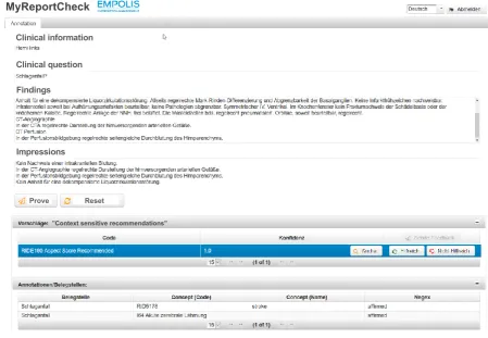
demonstrated the feasibility of our automated RadLex® framework (“MyReportCheck”, Figure
4) by comparing it to ML classifiers developed on human expert annotations. Furthermore, our
ensemble learning setup provides objective rankings and a generalizable blueprint for choosing
ML algorithms when developing classifiers for similar context-sensitive recommendation
tasks[62, 64].
Although reporting templates have been developed to promote and standardize the best practice
of radiological reporting[65-67], the majority of radiology reports are still created in free-text
format[68, 69]. This limits the use of radiology reports in clinical research and algorithm
development[63, 67, 69]. To overcome this, NLP pipelines including ML proved to be effective
to annotate and to extract recommendations from reports[69, 70]. Nonetheless, studies dealing
with ML algorithm development particularly for real-time context-sensitive assistance of
radiologists while writing reports are scarce[64, 71]. Therefore, in this work, we focused on
comprehensive and objective comparison of ML algorithms to provide technical guidance for
developing these algorithms on limited (non-English) training data. For this, we have put an
emphasis on the probabilistic evaluation and ranking of ML classifiers. This is less relevant for
biomarker CAR recommendation systems but crucial for automated inference systems for
We used a commercially available NLP pipeline that implements a common approach[8, 69]
comprised of cleansing, contextualization and concept recognition as well as negation detection
trained explicitly for German and English RadLex® mappings[1, 43]. This fully automated
approach to generate bag-of-RadLex mappings is advantageous compared to standard
BOW[35] approaches, as it already captures domain-specific knowledge including negation and
affirmation[3]. Mikolov et al. proposed word2vec to create semantic word embeddings, which
gained popularity in the field of radiology[5, 73]. However, word2vec struggles to properly
handle out-of-vocabulary words[74, 75]. Thus, it needs to be combined with radiology
domain-specific mappings. In contrast, our approach directly generates bag-of-RadLex terms for each
report. We then combine all binary RadLex® term occurrences in our corpus (separately for
findings and impressions) to generate the RadLex-DTMs. Therefore, our pipeline is also more
robust for new or missing words e.g. if a new report does not contain certain terms (present in
the training corpus), these can be easily substituted with 0 or new terms can be added to the
DTM and the ML classifier can be swiftly retrained. This commercial NLP-based
RadLex-mapping pipeline for creating DTMs is free for research purposes and can be easily utilized
through our Shiny application.
Similar to previous studies[65, 69], we also flattened the hierarchical tree structure of RadLex®
concepts and let the ML classifiers select subgroups of terms relevant to the classification task
automatically during training. For a similar domain-specific semantic-dictionary mapping, as
part of their hybrid word embedding model, Banerjee et al. created a custom ontology crawler
that identified key terms for pulmonary embolism[76]. Another approach by Percha et al.
included only partial flattening of RadLex®. They selected the eight most frequent parent
categories that were used to learn word and RadLex® term vector representations for
automatically expanding ontologies[5]. We have also found that certain key terms are missing
increase interoperability, aim to combine multiple (both radiology-specific and general
medical) ontologies or procedural databases such as RadLex®, LOINC/RSNA playbook, CDE
from the RSNA and Systematized Nomenclature of Medicine Clinical Terms (SNOMED CT)
as well as the International Classification of Diseases (v.10) Clinical Modification
(ICD-10-CM)[74, 77-79].
All investigated ML algorithms were “CPU only” thereby imposing minimal hardware
requirements and being quick both at train and test time[36]. These ML models have proven to
be effective on both text classification[34, 36, 80] and other high-dimensional medical problems
including high-throughput genomic microarray data[6, 81]. Additionally, we implemented a
nested CV learning framework in order to objectively assess the importance of each ML base
classifier and report section (i.e. findings and impressions) based on their probability estimates
of recommending ASPECTS[6]. Zinov et al. also used a probabilistic ensemble learning setup
to match lung nodule imaging features to text[71]. It is of note that there is multicollinearity
both on the level of RadLex® mappings when training ML base classifiers and when combining
the probability estimates of these ML classifiers on the second layer meta/ensemble-learner
level. Default settings of RF (both in Python and R) are less robust for these scenarios due to
the dilution of true features[6, 53, 55, 56]. To counter act dilution, we used the most robust
metric of permutation-based importance (type=1) without scaling for all RF models. In contrast,
boosted trees by design are less susceptible to correlation of features [42, 52]. The performance
of the investigated ML algorithms is differently sensitive to the number of features[6, 81].
Based on results by limiting the feature space with unsupervised variance filtering, we suggest
using all annotated RadLex® features as input and treating the number of features (p) as a
ML models developed on HEAF were similarly accurate (87%) to those developed on fully
automated cross-lingual RadLex® mappings (~85%), although the latter models had
substantially better calibration profiles (especially AUC and BS). This corresponded to results
by Tan et al. on lumbar spine imaging when comparing rule-based methods to ML models[82].
On the more heterogeneous and larger RadLex® feature space of the findings sections, most
ML models including fastText struggled but XGBoost performed best with an almost ideal
calibration profile among all models (including those developed on the impressions). As
impressions are expert-created condensed extracts of the most relevant information, ML
performed substantially better (all > 80%). Accordingly, both RF and XGBoost meta/ensemble
learners favored ML models that were developed on the impressions particularly fastText,
SVM-LK and BS-tuned RF. These second layer meta/ensemble models achieved precision of
90-93%, recall: 92-94% and F1 score: 91-93%, which was well in line with the performance of
information extraction model by Hassanpour et al. on a similarly sized (n=150) test set of
multi-institutional chest CT reports[69].
The advantage of RadLex-based ML models compared to fastText is that they contain
anatomical concepts and we can directly access negation information providing human
interpretable explanation of the model. For fastText, such concepts are not necessarily learnable
from limited training data or for more complex decision support scenarios other than
ASPECTS. This was also supported by the fact that, despite being a baseline model, single
CART performed remarkable well on the impressions implying that recommending ASPECTS
is a less complex decision task.
The present study has certain limitations as it was a single-center, retrospective cross-sectional
study of moderate size. Nonetheless, we selected a stratified random sample of ~200 reports
from ~4000 reports from a period of 4 years, which robustly represented the general daily
and ML algorithms and linear classifiers with respect to radiology-specific biomarker
(ASPECTS) recommendation tasks. Hence, there are natural extensions to our methodology
including the switch to well-known neural network architectures both to generate RadLex®
mappings[26, 83] and to create task-specific classifiers in an end-to-end manner such as
convolutional (CNN)[24], recurrent neural networks (RNN)[72] or long short-term memory
(LSTM) networks[63, 84]. However, fastText (with only a single hidden layer) has proven to
be on a par with these more complex network architectures on several benchmarks[36].
Although, incorporating pre-trained language-specific word representations into fastText was
expected to improve its accuracy we chose not to do so to allow for more direct performance
comparisons with bag-of-RadLex-based ML classifiers[58].
Utilizing large transformer architectures[25, 27-29, 85] directly on German free-text reports
would be a reasonable extension, however, sufficiently large non-English public radiology
domain-specific corpora for transfer learning are lacking and the interpretability of TLMs is
challenging[31]. Whether TLMs “truly learn” underlying concepts as a model of language or
just extract spurious statistical correlations is a topic of active research[32, 33]. Thus, our CT
stroke corpus can facilitate benchmarking of such models for the German radiological
domain[31, 83, 85].
For recommending ASPECTS we used pyes > 0.5 probability threshold. Optimizing this cutoff
could further improve the performance metrics of the ML classifiers – for example by
maximizing the Youden index[86].
To counteract class imbalance, we also explored upsampling, downsampling, random
over-sampling and synthetic minority over-over-sampling techniques (SMOTE)[87], however, they did
not improve the accuracy of ML classifiers on our data set (data not shown).
Regardless of these limitations, compared to text-based DL methods, our approach has some
major advantages: i) building ML classifiers on top of cross-lingual RadLex® mappings
labeled data – for which simple class labels are sufficient; ii) this approach can be easily adopted
to any other language where RadLex® was translated by the local radiological society; iii) an
ultimate benefit of our methodology is that it allows for the instant interoperability between
languages especially the direct transportability of any ML model created for biomarker
5. Conclusion
We showed that expert-based key information extraction and fully-automated RadLex
mapping-based machine learning is comparable and requires only a limited amount of
expert-labeled training data – even for highly imbalanced classification tasks. We performed detailed
comparative analyses of well-established ML algorithms and identified those, which are best
suited for automated rule learning on bag-of-RadLex® concepts (SVM, XGBoost and RF) and
directly on German radiology report texts (fastText) through utilizing a nested CV learning
framework.
Taken together, this work provides a generalizable probabilistic framework for developing
embedded ML algorithms for CAR tools to context-sensitively suggest, not just ASPECTS but
any required key biomarker information. Thereby improving report quality and facilitating
Data statement
Both the human expert annotated features (heaf.csv) and the fully automated NLP-based
RadLex® mappings (term-report-matrices) are provided in our GitHub repository
(https://github.com/mematt/ml4RadLexCAD/). The RadLex® annotation and scoring pipeline
(RASP) is freely available for research purposes as Shiny application at
www.mmatt.shinyapps.io/rasp . All tuned ML-model objects including the fold IDs for the 5 x
5-fold stratified nested CV scheme (nfolds.RData) are provided on GitHub. Additionally, we
provide R code for ML-model training and for generating calibration plots presented in Fig. 3.
Acknowledgements
Funding: M.E.M., C.G.C. and B.K. gratefully acknowledge funding from the German Federal
Ministry for Economic Affairs and Energy within the scope of Zentrales Innovationsprogramm
Mittelstand (ZF 4514602TS8). M.E.M., C.G.C., F.S., F.T. and T.G. were supported by funding
from the German Ministry for Education and Research (BMBF) within the framework of the
Medical Informatics Initiative (MIRACUM Consortium: Medical Informatics for Research and
Care in University Medicine; 01ZZ1801E).
Author contributions
M.E.M. conceptualized the study. A.G.J. and M.E.M. performed RIS data extraction and data
preparation. M.E.M., C.G.C. and H.W. analyzed the reports and performed expert feature
extraction. M.E.M. created the Shiny application. M.E.M. developed the machine learning
framework. A.G.J. applied the linear language models. B.K. developed the connection to the
RadLex® annotation service. F.S., F.T., V.S. and T.G. advised technical aspects of the study.
H.W. and M.E.M. supervised the clinical aspects of the study. M.E.M, B.K. and H.W. wrote
Declaration/Conflict of interest
B.K. is an employee of Empolis Information Management GmbH. M.E.M., C.G.C. and B.K.
received joint funding from the German Federal Ministry for Economic Affairs and Energy
within the scope of Zentrales Innovationsprogramm Mittelstand. The founding sponsors had no
role in the design of the study; in the collection, analyses, or interpretation of data; in the writing
of the manuscript; and in the decision to publish the results. The other authors declare no
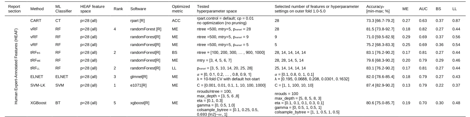
Table 1 | Summary table of performance measures of the investigated ML algorithms developed on human expert-annotated features (HEAF).
Report
section Method ML Classifier
HEAF feature
space Rank Software
Optimized metric
Tested
hyperparameter space
Selected number of features or hyperparameter settings on outer fold 1.0-5.0
Accuracy#
[min-max; %] ME AUC BS LL
H u m a n E x p e rt -A n n o ta te d F e a tu re s (H E A F )
CART CT p=28 (all) rpart [R] ACC rpart.control = default; cp = 0.01
no optimization (no pruning) 28 73.3 [66.7-79.2] 0.27 0.63 0.37 0.87
vRF RF p=28 (all) 4 randomForest [R] ME ntree =500, mtry=5, pvarsel = 28 28 81.5 [73.8-92.7] 0.18 0.82 0.27 0.44
vRF RF p=28 (all) randomForest[R] ME ntree =500, mtry=5, pvarsel = 9 9 71.0 [59.5-82.9] 0.29 0.69 0.37 0.56
vRF RF p=28 (all) randomForest[R] ME ntree =500, mtry=5, pvarsel = 5 5 75.2 [68.3-83.3] 0.25 0.69 0.36 0.54
tRFBS RF p=28 (all) 2 randomForest[R] BS ntree = [100, 200, 300, … , 900, 1000] 28, 14, 14, 14, 14 83.1 [76.2-90.2] 0.17 0.81 0.27 0.44
tRFME RF p=28 (all) randomForest[R] ME mtry = [3, 4, 5, 6, 7] 28, 28, 14, 5, 14 79.6 [68.3-90.2] 0.20 0.79 0.29 0.46
tRFLL RF p=28 (all) 2 randomForest[R] LL pvarsel = [3, 5, 10, 14, 20, 25, 28] 25, 14, 14, 14, 14 83.1 [76.2-90.2] 0.17 0.81 0.27 0.44
ELNET ELNET p=28 (all) 3 glmnet[R] ME λ = 10-fold CV with default hot-start 𝛼 = [0, 0.1, 0.2, … , 0.8, 0.9, 1] 𝛼λ = [0.195, 0.0688, 0.208, 0.0301, 0.1632] = [0.1, 0.8, 0, 1, 0.1] 82.0 [78.6-85.4] 0.18 0.79 0.27 0.43
SVM-LK SVM p=28 (all) 1 e1071[R] ME C = [0.001, 0.01, 0.1, 1, 10, 100, 1000] C = [1, 1, 100, 10, 10] 87.4 [82.9-90.2] 0.13 0.79 0.22 0.37
XGBoost BT p=28 (all) 5 xgboost[R] ME
nrouds/ntree = 100, max_depth = [3, 5, 6 ,8] eta = [0.1, 0.3] gamma = [0, 0.5, 1.0]
colsample_bytree = [0.1, 0.25, 0.5, 0.693 (ln2)~RF, 1]
nrouds = 100
max_depth = [5, 8, 5, 8, 3] eta = [0.1, 0.1, 0.1, 0.3, 0.1] gamma = [0, 0.5, 1, 0.5, 1] colsample_bytree = [1, 1, 0.5, 1, 0.5]
80.6 [75.0-85.7] 0.19 0.70 0.30 0.48
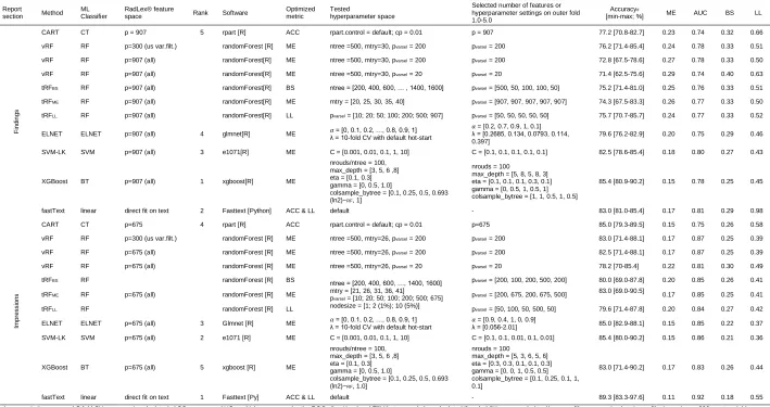
Table 2 | Summary table of performance measures of the investigated ML algorithms on the NLP-annotated bag-of-RadLex® features of the findings and impressions sections.
Report
section Method ML Classifier
RadLex® feature
space Rank Software
Optimized metric
Tested
hyperparameter space
Selected number of features or hyperparameter settings on outer fold 1.0-5.0
Accuracy#
[min-max; %] ME AUC BS LL
F in d in g s
CART CT p = 907 5 rpart [R] ACC rpart.control = default; cp = 0.01 p = 907 77.2 [70.8-82.7] 0.23 0.74 0.32 0.66
vRF RF p=300 (us var.filt.) randomForest [R] ME ntree =500, mtry=30, pvarsel = 200 pvarsel = 200 76.2 [71.4-85.4] 0.24 0.78 0.33 0.51
vRF RF p=907 (all) randomForest[R] ME ntree =500, mtry=30, pvarsel = 200 pvarsel = 200 72.8 [67.5-78.6] 0.27 0.78 0.33 0.50
vRF RF p=907 (all) randomForest[R] ME ntree =500, mtry=30, pvarsel = 20 pvarsel = 20 71.4 [62.5-75.6] 0.29 0.74 0.40 0.63
tRFBS RF p=907 (all) randomForest[R] BS ntree = [200, 400, 600, … , 1400, 1600] pvarsel = [500, 50, 100, 100, 50] 75.2 [71.4-81.0] 0.25 0.76 0.33 0.51
tRFME RF p=907 (all) randomForest[R] ME mtry = [20, 25, 30, 35, 40] pvarsel = [907, 907, 907, 907, 907] 74.3 [67.5-83.3] 0.26 0.77 0.33 0.50
tRFLL RF p=907 (all) randomForest[R] LL pvarsel = [10; 20; 50; 100; 200; 500; 907] pvarsel = [50, 50, 50, 50, 50] 75.7 [70.7-85.7] 0.24 0.77 0.33 0.52
ELNET ELNET p=907 (all) 4 glmnet[R] ME 𝛼λ = 10-fold CV with default hot-start = [0, 0.1, 0.2, …, 0.8, 0.9, 1]
𝛼 = [0.2, 0.7, 0.9, 1, 0.1] λ = [0.2685, 0.134, 0.0793, 0.114, 0.397]
79.6 [76.2-82.9] 0.20 0.75 0.29 0.46
SVM-LK SVM p=907 (all) 3 e1071[R] ME C = [0.001, 0.01, 0.1, 1, 10] C = [0.1, 0.1, 0.1, 0.1, 0.1] 82.5 [78.6-85.4] 0.18 0.80 0.27 0.43
XGBoost BT p=907 (all) 1 xgboost[R] ME
nrouds/ntree = 100, max_depth = [3, 5, 6 ,8] eta = [0.1, 0.3] gamma = [0, 0.5, 1.0]
colsample_bytree = [0.1, 0.25, 0.5, 0.693 (ln2)~RF, 1]
nrouds = 100
max_depth = [5, 8, 5, 8, 3] eta = [0.1, 0.1, 0.1, 0.3, 0.1] gamma = [0, 0.5, 1, 0.5, 1] colsample_bytree = [1, 1, 0.5, 1, 0.5]
85.4 [80.9-90.2] 0.15 0.78 0.25 0.45
fastText linear direct fit on text 2 Fasttext [Python] ACC & LL default - 83.0 [81.0-85.4] 0.17 0.81 0.29 0.98
Imp re ssi o n s
CART CT p=675 4 rpart [R] ACC rpart.control = default; cp = 0.01 p=675 85.0 [79.3-89.5] 0.15 0.75 0.26 0.58
vRF RF p=300 (us var.filt.) randomForest [R] ME ntree =500, mtry=26, pvarsel = 200 pvarsel = 200 83.0 [71.4-88.1] 0.17 0.87 0.25 0.39
vRF RF p=675 (all) randomForest [R] ME ntree =500, mtry=26, pvarsel = 200 pvarsel = 200 82.5 [71.4-88.1] 0.17 0.87 0.25 0.39
vRF RF p=675 (all) randomForest [R] ME ntree =500, mtry=26, pvarsel = 20 pvarsel = 20 78.2 [70-85.4] 0.22 0.81 0.30 0.49
tRFBS RF
p=675 (all)
randomForest [R] BS ntree = [200, 400, 600, …, 1400, 1600]
mtry = [21, 26, 31, 36, 41]
pvarsel = [10; 20; 50; 100; 200; 500; 675] nodesize = [1; 2 (1%); 10 (5%)]
pvarsel = [200, 100, 200, 500, 200] 80.0 [69.0-87.8] 0.20 0.85 0.26 0.41
tRFME RF randomForest [R] ME pvarsel = [200, 675, 200, 675, 500] 83.0 [69.0-90.5] 0.17 0.85 0.25 0.41
tRFLL RF randomForest [R] LL pvarsel = [50, 100, 50, 500, 50] 79.6 [71.4-87.8] 0.20 0.84 0.27 0.42
ELNET ELNET p=675 (all) 3 Glmnet [R] ME 𝛼 = [0, 0.1, 0.2, …, 0.8, 0.9, 1]
λ = 10-fold CV with default hot-start 𝛼
= [0.9, 0.4, 1, 0, 0.9]
λ = [0.056-2.01] 85.0 [82.9-88.1] 0.15 0.85 0.22 0.37 SVM-LK SVM p=675 (all) 2 e1071 [R] ME C = [0.001, 0.01, 0.1, 1, 10] C = [0.1, 0.1, 0.01, 0.1, 0.01] 85.4 [80.0-90.2] 0.15 0.86 0.21 0.36
XGBoost BT p=675 (all) 5 xgboost [R] ME
nrouds/ntree = 100, max_depth = [3, 5, 6 ,8] eta = [0.1, 0.3] gamma = [0, 0.5, 1.0]
colsample_bytree = [0.1, 0.25, 0.5, 0.693 (ln2)~RF, 1.0]
nrouds = 100
max_depth = [5, 3, 6, 5, 6] eta = [0.3, 0.3, 0.1, 0.1, 0.3] gamma = [0, 0, 1, 0.5, 0.5] colsample_bytree = [0.1, 0.25, 0.1, 1, 0.1]
83.0 [71.4-90.2] 0.17 0.83 0.26 0.44
fastText linear direct fit on text 1 Fasttext [Py] ACC & LL default - 89.3 [83.3-97.6] 0.11 0.92 0.18 0.55
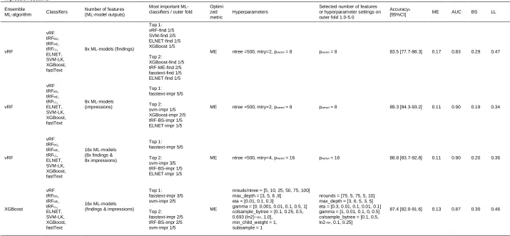
Table 3 | Summary table of performance measures of the second layer meta/ensemble learners (random forests and boosted trees) combining the predictions of all RadLex®-based ML base classifiers from the findings and impression sections.
Ensemble
ML-algorithm Classifiers
Number of features (ML-model outputs)
Most important ML-classifiers / outer fold
Optimi zed metric
Hyperparameters
Selected number of features or hyperparameter settings on outer fold 1.0-5.0
Accuracy#
[95%CI] ME AUC BS LL
vRF vRF tRFBS, tRFME, tRFLL, ELNET, SVM-LK, XGBoost, fastText
8x ML-models (findings)
Top 1: vRF-find 1/5 SVM-find 2/5 ELNET-find 1/5 XGBoost 1/5 Top 2: XGBoost-find 1/5 tRF-ME-find 2/5 fasstext-find 1/5 ELNET-find 1/5
ME ntree =500, mtry=2, pvarsel = 8 pvarsel = 8 83.5 [77.7-88.3] 0.17 0.83 0.29 0.47
vRF vRF tRFBS, tRFME, tRFLL, ELNET, SVM-LK, XGBoost, fastText 8x ML-models (impressions) Top 1: fasstext-impr 5/5 Top 2: svm-impr 1/5 XGBoost-impr 2/5 tRF-BS-impr 1/5 ELNET-impr 1/5
ME ntree =500, mtry=2, pvarsel = 8 pvarsel = 8 89.3 [84.3-93.2] 0.11 0.90 0.19 0.34
vRF vRF tRFBS, tRFME, tRFLL, ELNET, SVM-LK, XGBoost, fastText 16x ML-models (8x findings & 8x impressions) Top 1: fasstext-impr 5/5 Top 2: svm-impr 3/5 tRF-BS-impr 1/5 ELNET-impr 1/5
ME ntree =500, mtry=4, pvarsel = 16 pvarsel = 16 88.8 [83.7-92.8] 0.11 0.90 0.20 0.36
XGBoost vRF tRFBS, tRFME, tRFLL, ELNET, SVM-LK, XGBoost, fastText 16x ML-models (findings & impressions)
Top 1: fasstext-impr 3/5 svm-impr 2/5 Top 2: fasstext-impr 2/5 tRF-BS-impr 2/5 svm-impr 1/5 ME
nrouds/ntree = [5, 10, 25, 50, 75, 100] max_depth = [3, 5, 6 ,8]
eta = [0.01, 0.1, 0.3]
gamma = [0, 0.001, 0.01, 0.1, 0.5, 1] colsample_bytree = [0.1, 0.25, 0.5, 0.693 (ln2)~RF, 1.0],
min_child_weight = 1, subsample = 1
nrounds = [75, 5, 75, 5, 10] max_depth = [3, 6, 5, 3, 5] eta = [0.3, 0.01, 0.1, 0.01, 0.1] gamma = [1, 0.01, 0.1, 0, 0.5] colsample_bytree = [0.1, 0.5, ln2~RF, 0.1, 0.25]
87.4 [82.0-91.6] 0.13 0.87 0.30 0.46
References:
[1] F. Jungmann, B. Kämpgen, P. Mildenberger, I. Tsaur, T. Jorg, C. Düber, P. Mildenberger, R. Kloeckner, Towards data-driven medical imaging using natural language processing in patients with suspected urolithiasis, International Journal of Medical Informatics (2020) 104106.
[2] P.A. Barber, A.M. Demchuk, J. Zhang, A.M. Buchan, Validity and reliability of a quantitative computed tomography score in predicting outcome of hyperacute stroke before thrombolytic therapy. ASPECTS Study Group. Alberta Stroke Programme Early CT Score, Lancet 355(9216) (2000) 1670-4.
[3] C.P. Langlotz, RadLex: a new method for indexing online educational materials, Radiographics : a review publication of the Radiological Society of North America, Inc 26(6) (2006) 1595-7.
[4] R.S.o.N. America, RadLex radiology lexicon. http://www.radlex.org/. (Accessed 11.11.2019 2019).
[5] B. Percha, Y. Zhang, S. Bozkurt, D. Rubin, R.B. Altman, C.P. Langlotz, Expanding a radiology lexicon using contextual patterns in radiology reports, Journal of the American Medical Informatics Association : JAMIA 25(6) (2018) 679-685. [6] M.E. Maros, D. Capper, D.T.W. Jones, V. Hovestadt, A. von Deimling, S.M. Pfister, A. Benner, M. Zucknick, M. Sill,
Machine learning workflows to estimate class probabilities for precision cancer diagnostics on DNA methylation microarray data, Nature Protocols 15(2) (2020) 479-512.
[7] M.D. Mamlouk, P.C. Chang, R.R. Saket, Contextual Radiology Reporting: A New Approach to Neuroradiology Structured Templates, AJNR Am J Neuroradiol 39(8) (2018) 1406-1414.
[8] E. Pons, L.M. Braun, M.G. Hunink, J.A. Kors, Natural Language Processing in Radiology: A Systematic Review, Radiology 279(2) (2016) 329-43.
[9] E.J. Topol, High-performance medicine: the convergence of human and artificial intelligence, Nature Medicine 25(1) (2019) 44-56.
[10] J.J. Titano, M. Badgeley, J. Schefflein, M. Pain, A. Su, M. Cai, N. Swinburne, J. Zech, J. Kim, J. Bederson, J. Mocco, B. Drayer, J. Lehar, S. Cho, A. Costa, E.K. Oermann, Automated deep-neural-network surveillance of cranial images for acute neurologic events, Nature Medicine 24(9) (2018) 1337-1341.
[11] D.J. Vreeman, S. Abhyankar, K.C. Wang, C. Carr, B. Collins, D.L. Rubin, C.P. Langlotz, The LOINC RSNA radiology playbook - a unified terminology for radiology procedures, Journal of the American Medical Informatics Association : JAMIA 25(7) (2018) 885-893.
[12] D.L. Rubin, C.E. Kahn, Jr., Common Data Elements in Radiology, Radiology 283(3) (2017) 837-844.
[13] M. Goyal, B.K. Menon, W.H. van Zwam, D.W. Dippel, P.J. Mitchell, A.M. Demchuk, A. Davalos, C.B. Majoie, A. van der Lugt, M.A. de Miquel, G.A. Donnan, Y.B. Roos, A. Bonafe, R. Jahan, H.C. Diener, L.A. van den Berg, E.I. Levy, O.A. Berkhemer, V.M. Pereira, J. Rempel, M. Millan, S.M. Davis, D. Roy, J. Thornton, L.S. Roman, M. Ribo, D. Beumer, B. Stouch, S. Brown, B.C. Campbell, R.J. van Oostenbrugge, J.L. Saver, M.D. Hill, T.G. Jovin, Endovascular thrombectomy after large-vessel ischaemic stroke: a meta-analysis of individual patient data from five randomised trials, Lancet 387(10029) (2016) 1723-31.
[14] A. Gerstmair, P. Daumke, K. Simon, M. Langer, E. Kotter, Intelligent image retrieval based on radiology reports, European radiology 22(12) (2012) 2750-2758.
[15] D. Pinto Dos Santos, B. Baessler, Big data, artificial intelligence, and structured reporting, European radiology experimental 2(1) (2018) 42.
[16] A. Rajkomar, E. Oren, K. Chen, A.M. Dai, N. Hajaj, M. Hardt, P.J. Liu, X. Liu, J. Marcus, M. Sun, Scalable and accurate deep learning with electronic health records, NPJ Digital Medicine 1(1) (2018) 18.
[17] A. Rajkomar, J. Dean, I. Kohane, Machine Learning in Medicine, New England Journal of Medicine 380(14) (2019) 1347-1358.
[18] N. Westhoff, F. Siegel, C. Peter, S. Hetjens, S. Porubsky, T. Martini, J. von Hardenberg, M.S. Michel, J. Budjan, M. Ritter, Defining the target prior to prostate fusion biopsy: the effect of MRI reporting on cancer detection, World journal of urology 37(2) (2019) 327-335.
[19] E.S. Burnside, E.A. Sickles, L.W. Bassett, D.L. Rubin, C.H. Lee, D.M. Ikeda, E.B. Mendelson, P.A. Wilcox, P.F. Butler, C.J. D'Orsi, The ACR BI-RADS experience: learning from history, J Am Coll Radiol 6(12) (2009) 851-60.
[20] Y. Hong, C.E. Kahn, Jr., Content analysis of reporting templates and free-text radiology reports, J Digit Imaging 26(5) (2013) 843-9.
[21] C.E. Kahn Jr, C.P. Langlotz, E.S. Burnside, J.A. Carrino, D.S. Channin, D.M. Hovsepian, D.L. Rubin, Toward best practices in radiology reporting, Radiology 252(3) (2009) 852-856.
[22] G. Choy, O. Khalilzadeh, M. Michalski, S. Do, A.E. Samir, O.S. Pianykh, J.R. Geis, P.V. Pandharipande, J.A. Brink, K.J. Dreyer, Current Applications and Future Impact of Machine Learning in Radiology, Radiology 288(2) (2018) 318-328. [23] R.C. Mayo, J. Leung, Artificial intelligence and deep learning - Radiology's next frontier?, Clinical imaging 49 (2018)
87-88.
[24] M.C. Chen, R.L. Ball, L. Yang, N. Moradzadeh, B.E. Chapman, D.B. Larson, C.P. Langlotz, T.J. Amrhein, M.P. Lungren, Deep Learning to Classify Radiology Free-Text Reports, Radiology 286(3) (2018) 845-852.
[25] J. Devlin, M.-W. Chang, K. Lee, K. Toutanova, Bert: Pre-training of deep bidirectional transformers for language understanding, arXiv preprint arXiv:1810.04805 (2018).
[26] M.E. Peters, M. Neumann, M. Iyyer, M. Gardner, C. Clark, K. Lee, L. Zettlemoyer, Deep contextualized word representations, arXiv preprint arXiv:1802.05365 (2018).
[27] A. Radford, K. Narasimhan, T. Salimans, I. Sutskever, Improving language understanding by generative pre-training, URL
https://s3-us-west-2. amazonaws. com/openai-assets/researchcovers/languageunsupervised/language understanding paper. pdf (2018).
[29] M. Shoeybi, M. Patwary, R. Puri, P. LeGresley, J. Casper, B. Catanzaro, Megatron-lm: Training multi-billion parameter language models using gpu model parallelism, arXiv preprint arXiv:1909.08053 (2019).
[30] P. Richter-Pechanski, S. Riezler, C. Dieterich, De-Identification of German Medical Admission Notes, GMDS, 2018, pp. 165-169.
[31] B. Heinzerling, NLP's Clever Hans Moment has Arrived, 2019. https://thegradient.pub/nlps-clever-hans-moment-has-arrived/. (Accessed August 26, 2019 2019).
[32] T. Niven, H.-Y. Kao, Probing neural network comprehension of natural language arguments, arXiv preprint arXiv:1907.07355 (2019).
[33] C. Wang, M. Li, A.J. Smola, Language models with transformers, arXiv preprint arXiv:1904.09408 (2019).
[34] C.D. Manning, P. Raghavan, H. Schütze, Introduction to information retrieval, Cambridge university press Cambridge2008.
[35] M.E. Maros, R. Wenz, A. Forster, M.F. Froelich, C. Groden, W.H. Sommer, S.O. Schonberg, T. Henzler, H. Wenz, Objective Comparison Using Guideline-based Query of Conventional Radiological Reports and Structured Reports, In Vivo 32(4) (2018) 843-849.
[36] A. Joulin, E. Grave, P. Bojanowski, T. Mikolov, Bag of tricks for efficient text classification, arXiv preprint arXiv:1607.01759 (2016).
[37] L. Breiman, Random forests, Machine learning 45(1) (2001) 5-32.
[38] H. Zou, T. Hastie, Regression shrinkage and selection via the elastic net, with applications to microarrays, JR Stat Soc Ser B 67 (2003) 301-20.
[39] J. Friedman, T. Hastie, R. Tibshirani, Regularization paths for generalized linear models via coordinate descent, Journal of statistical software 33(1) (2010) 1.
[40] C. Cortes, V. Vapnik, Support-vector networks, Machine learning 20(3) (1995) 273-297.
[41] L. Breiman, J. Friedman, C. Stone, R. Olshen, Classification and regression trees., Chapman and Hall/CRC press, 1984. [42] T. Chen, T. He, Xgboost: extreme gradient boosting, R package version 0.4-2 (2016).
[43] F. Jungmann, S. Kuhn, I. Tsaur, B. Kämpgen, Natural Language Processing in der Radiologie, Der Radiologe 59(9) (2019) 828-832.
[44] M. Wintermark, P.C. Sanelli, G.W. Albers, J. Bello, C. Derdeyn, S.W. Hetts, M.H. Johnson, C. Kidwell, M.H. Lev, D.S. Liebeskind, H. Rowley, P.W. Schaefer, J.L. Sunshine, G. Zaharchuk, C.C. Meltzer, Imaging recommendations for acute stroke and transient ischemic attack patients: A joint statement by the American Society of Neuroradiology, the American College of Radiology, and the Society of NeuroInterventional Surgery, AJNR Am J Neuroradiol 34(11) (2013) E117-27. [45] D. Deutsche Gesellschaft für Neurologie, Diagnostic of acute cerebrovascular diseases AWMF-030/117 2016.
https://www.awmf.org/leitlinien/detail/ll/030-117.html. (Accessed Jan 1, 2020.
[46] V. Cotik, R. Roller, F. Xu, H. Uszkoreit, K. Budde, D. Schmidt, Negation detection in clinical reports written in German, Proceedings of the Fifth Workshop on Building and Evaluating Resources for Biomedical Text Mining (BioTxtM2016), 2016, pp. 115-124.
[47] S. Robertson, H. Zaragoza, The probabilistic relevance framework: BM25 and beyond, Foundations and Trends® in Information Retrieval 3(4) (2009) 333-389.
[48] V.I. Levenshtein, Binary codes capable of correcting deletions, insertions, and reversals, Soviet physics doklady, 1966, pp. 707-710.
[49] P. Kluegl, M. Toepfer, P.-D. Beck, G. Fette, F. Puppe, UIMA Ruta: Rapid development of rule-based information extraction applications, Natural Language Engineering 22(1) (2016) 1-40.
[50] L. Breiman, Classification and regression trees, Routledge2017.
[51] L. Breiman, P. Spector, Submodel Selection and Evaluation in Regression. The X-Random Case, International Statistical Review / Revue Internationale de Statistique 60(3) (1992) 291-319.
[52] T. Hastie, R. Tibshirani, J. Friedman, The elements of statistical learning: Data Mining, Inference and Prediction, 2. ed., Springer, New York, NY2009.
[53] A. Liaw, M. Wiener, Classification and regression by randomForest, R news 2(3) (2002) 18-22.
[54] C. Chen, A. Liaw, L. Breiman, Using random forest to learn imbalanced data, University of California, Berkeley 110 (2004).
[55] C. Strobl, A.-L. Boulesteix, A. Zeileis, T. Hothorn, Bias in random forest variable importance measures: Illustrations, sources and a solution, BMC bioinformatics 8(1) (2007) 1.
[56] T. Parr, K. Turgutlu, C. Csiszar, J. Howard, Beware Default Random Forest Importances, 2018. https://explained.ai/rf-importance/.
[57] A. Paluszynska, P. Biecek, Y. Jiang, randomForestExplainer: Explaining and Visualizing Random Forests in Terms of Variable Importance, version 0.10. 0, R package (2019).
[58] E. Grave, P. Bojanowski, P. Gupta, A. Joulin, T. Mikolov, Learning word vectors for 157 languages, arXiv preprint arXiv:1802.06893 (2018).
[59] M.H. DeGroot, S.E. Fienberg, The comparison and evaluation of forecasters, The statistician (1983) 12-22. [60] D. Nee, Calibrating classifier probabilities Website, Blog., 2014.
[61] A. Niculescu-Mizil, R. Caruana, Predicting good probabilities with supervised learning, Proceedings of the 22nd international conference on Machine learning, ACM, Bonn, Germany, 2005, pp. 625-632.
[62] M. Kohli, T. Alkasab, K. Wang, M.E. Heilbrun, A.E. Flanders, K. Dreyer, C.E. Kahn, Jr., Bending the Artificial Intelligence Curve for Radiology: Informatics Tools From ACR and RSNA, J Am Coll Radiol 16(10) (2019) 1464-1470. [63] R.C. Carlos, C.E. Kahn, S. Halabi, Data Science: Big Data, Machine Learning, and Artificial Intelligence, Journal of the
American College of Radiology 15(3, Part B) (2018) 497-498.
[64] T. Syeda-Mahmood, Role of Big Data and Machine Learning in Diagnostic Decision Support in Radiology, Journal of the American College of Radiology 15(3, Part B) (2018) 569-576.
[66] C.E. Kahn, Jr., M.E. Heilbrun, K.E. Applegate, From guidelines to practice: how reporting templates promote the use of radiology practice guidelines, J Am Coll Radiol 10(4) (2013) 268-73.
[67] T.A. Morgan, M.E. Helibrun, C.E. Kahn, Jr., Reporting initiative of the Radiological Society of North America: progress and new directions, Radiology 273(3) (2014) 642-5.
[68] D.L. Weiss, C.P. Langlotz, Structured reporting: patient care enhancement or productivity nightmare?, Radiology 249(3) (2008) 739-47.
[69] S. Hassanpour, C.P. Langlotz, Information extraction from multi-institutional radiology reports, Artificial intelligence in medicine 66 (2016) 29-39.
[70] M. Yetisgen-Yildiz, M.L. Gunn, F. Xia, T.H. Payne, A text processing pipeline to extract recommendations from radiology reports, Journal of Biomedical Informatics 46(2) (2013) 354-362.
[71] D. Zinovev, D. Raicu, J. Furst, S.G. Armato III, Predicting radiological panel opinions using a panel of machine learning classifiers, Algorithms 2(4) (2009) 14