Design And Implementation Of Cnn Adaptive Single Image Gradient Learner For Image Contrast Enhancement

3861 IJSTR©2020

Design And Implementation Of Cnn Adaptive

Single Image Gradient Learner For Image

Contrast Enhancement

Abstract: Due to camera resolution or any lighting condition, captured image are generally over-exposed or under-exposed conditions. So, there is need of some enhancement techniques that improvise these artifacts from recorded pictures or images. So, the objective of image enhancement and adjustment techniques is to improve the quality and characteristics of an image. In general terms, the enhancement of image distorts the original numerical values of an image. Therefore, it is required to design such enhancement technique that do not compromise with the quality of the image. Many research work have been done in this field. One among them is SICE methodology. Most of the existing SICE methods, adjust the tone curve to correct the contrast of an input image. But SICE doesn’t work efficiently due to limited amount of information contained in a single image. In this paper, the Convolutional Neural Network (CNN) Adaptive Single Image Gradient Learner is proposed. By applying this technique, the input low contrast images are capable to adapt according to high quality enhancement accordingly over-exposed or underexposed input image. The result analysis shows that the developed CNN Adaptive Single Image Gradient Learner significantly advantages over existing methods.

Index Terms: Digital Image Processing, Image Enhancement, CNN, PSNR, FSIM.

——————————  ——————————

1.

INTRODUCTION

In image processing applications, one of the main preprocessing phases is image enhancement that is used to produce high quality image or enhanced image than the original input image. These enhanced images can be used in many applications such as remote sensing applications, geo-satellite images, etc. The quality of an image are affected due to several conditions such as by poor illumination, atmospheric condition, wrong lens aperture setting of the camera, noise, etc [2]. So, such degraded/low exposure images are needed to be enhanced by increasing the brightness as well as its contrast and this can be possible by the method of image enhancement. The image enhancement techniques are divided into two types, one is spatial techniques and other is frequency domain image enhancement [1]. In spatial domain image enhancement methodology, the pixels of an image enhance themselves directly in order to improve the image quality. Whereas in frequency domain image enhancement techniques, frequency transformation is performed on the pixel intensity values for their enhancement. Many research works have been done in the field of image enhancement Some of them are good in contrast enhancement and some are helpful in image denoising. While designing image enhancement technique, it should be focused that, the technique should capable of enhancing real color images in less time as well as with less computational cost. This can be achieved by reducing following factors:

i. Effect caused due to fog or haze environment. ii. Uneven illumination effect on an image. iii. Addition of noise in an image.

In this paper, the work is focused on contrast enhancement of an low exposure image. Before designing the image enhancement methodology following objectives need to be fulfilled:

i. The proposed methodology should be adaptive to any type of images.

ii. Processing time should be less.

iii. Computational overhead or resources should also be less.

The outline of the paper is stated as: In section II brief description of image enhancement methodology is discussed. In section III Database Description is given. In section IV performance parameters are discussed. Section V discusses the result analysis and compared the performance of proposed methodology with the existing approaches. Section VI concludes with the performance of proposed CNN Adaptive Single Image Gradient Learner.

2.

METHODOLOGY

In this technology era, there are several improvements as well as developments in the field of image sensors and cameras. In near future, this technology will be as much developed that how human visual system perceives natural scenes, cameras can capture similar images. However, the range of light intensity that any camera can capture is in between 28 ₋₂14_. This intensity is measured in term stop which is base 2 logarithm of the dynamic range. It is known that the DSLR camera can capture with an about 8 to 12 stops dynamic range whereas the human visual system can perceive the dynamic range more than 24 stops. With the high dynamic range of the camera, there may causes the underexposed as well as over-exposed conditions which needs to be adjusted [3]. The dynamic range of the cameras are quite low as compared to the natural scenes.

_______________________________

• Deepanjali titariya is currently pursuing masters of engineering program in Department of computer science engineering in UIT Rajiv Gandhi Proudyogiki vishwavidyalaya, Bhopal, India, PH-9407534037. E-mail : [email protected]

• Rajeev PAndey is currently working as a Assistant Professor in Department of computer science engineering in UIT Rajiv Gandhi Proudyogiki vishwavidyalaya, Bhopal, India, PH-9479907881. E-mail: [email protected]

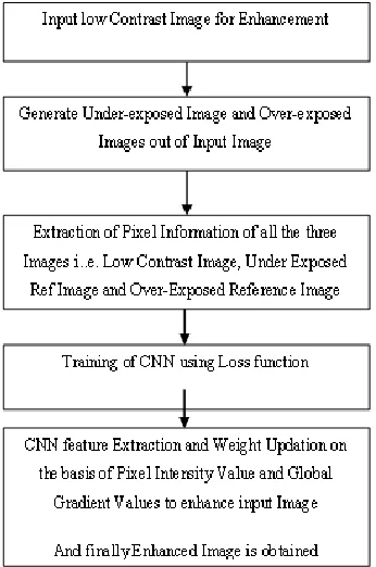
3862 Figure 1: Flowchart of Proposed Methodology

In order to gain above mentioned objectives in section I, in this paper, images are collected with low-exposure image sequences of natural scenes.

Following Steps are performed while enhancing the contrast of images:

Step 1: Input the low contrast image

Step 2: Generation of Under-exposed Image and Over-exposed Images out of Input Low Contrast Image and considered it as Reference Images

Step 3: Extraction of Pixel Component out of low contrast image as well as from both reference images

Step 4: Training the proposed CNN network and generate CNN features with smallest DSSIM loss function

Step 5: Updation of low contrast image pixel intensity as well as global gradient value according to CNN features

Step 6: Evaluation of Performance Parameters such as FSSIM and PSNR values.

The details of all the steps are described as follows:

A. Data Collection

In order to design robust and efficient low contrast image enhancement technique, it is required to collect input images from real-world natural scene. In this paper, different image sequences are collected from different camera and collected as a common dataset. For creating low contrast image dataset, the exposure value of the camera are set and collected different sequences of indoor and outdoor scenes. After collecting the low contrast input images, under exposed and over exposed images are created by manipulating the exposure value and save as a reference images.

B. Reference Image Generation

For reference image generation, HDR algorithm is used to

generate under exposed and over exposed high quality reference images.

C. CNN Adaptive Single Image Gradient Learner

The traditional single image contrast enhancement techniques (SICE) is based on histogram equalization which increases the intensity value of the pixels by distributing or equalizing the intensity value of image according to the neighboring pixel values. This illuminates the intensity value of the low contrast image. However, SICE algorithm is not quite efficient to generate high quality image with respect to low contrast images just due to complex background intensity values in the natural scene images.

With the constructed dataset, the proposed work will designed a CNN Adaptive Single Image Gradient Learner to know and map a equalization function among low contrast image I(x, y) and its respective reference images Irefunder-exposed (x, y) and Irefover-exposed (x, y). Further, the work is proceeded to train a CNN network accordingly loss function i.e. Structural dissimilarity (DSSIM).

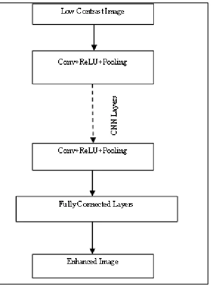
D. CNN Network Architecture

The proposed CNN has 5 convolutional layers and 3 fully connected layer which are shown in Figure 2.

i. Conv with 96 filters of size 11*11 with strides 4 are used to generate 96 feature maps

ii. For nonlinearity in network, ReLU (Rectified Linear Unit) is applied.

iii. Max Pooling with 3*3 with stride 2

iv. Conv with 256 filters of size 5*5 with 1 stride that generate 256 feature maps

v. For nonlinearity in network, ReLU (Rectified Linear Unit) is applied.

vi. Max Pooling with 3*3 with stride 2

vii. Conv with 384 filters of size 3*3 with 1 stride that generate 384 feature maps

viii. For nonlinearity in network, ReLU (Rectified Linear Unit) is applied.

ix. Max Pooling with 3*3 with stride 2

x. Conv with 384 filters of size 3*3 with 1 stride that generate 384 feature maps

xi. For nonlinearity in network, ReLU (Rectified Linear Unit) is applied.

xii. Conv with 256 filters of size 3*3 with 1 stride that generate 256 feature maps

xiii. For nonlinearity in network, ReLU (Rectified Linear Unit) is applied.

xiv. Max Pooling with 3*3 with stride 2

xv. Fully connected layer with 4096 neurons each for adding the operation that is used to attach the feature maps.

The basic idea of the CNN architecture is as follows:

i. Copy convolution layers into different GPUs

ii. Distribute the fully connected layers into different GPUs.

iii. Feed one batch of training data into convolutional layers for every GPU (Data Parallel).

3863 IJSTR©2020

E. Stride Convolution

The feature map generated according to the network is reduced by the convolutional operations. Padding is done to the output images before performing convolution, as output image has to be of same size as that of input image [5]. But this padding may cause artifact in the input image. So, this network is designed with deconvolution layer to make the output size be similar to input size. This deconvolution layer not only decreases the artifacts as well as reduces the computational overhead by applying filters.

Figure 2: Proposed CNN Architecture

F. Rectified Linear Unit

Rectified Linear Unit (ReLU) are used in many CNN architectures as an activation function for the network. In this activation function, the negative co-efficient are replaced with zero value which is represented by the local features of the input image. The function is represented as:

𝑓(𝑥) = {0 𝑓𝑜𝑟 𝑥 < 0

𝑥 𝑓𝑜𝑟 𝑥 ≥ 0 }

Some of the neurons dropped because they do not contribute to forward passage and do not participate in backpropagation. Every time an input is presented, the neural network analyzes another architecture, but all these architectures share a common weight. This technique reduces the complex adaptations of neurons because a neuron cannot rely on the presence of some other neurons. The proposed CNN Adaptive Single Image Gradient Learner is designed to enhance the contrast of the input image I(x,y) with respect to the reference images by learning the mapping function between the luminance component of the input low-contrast image and the luminance component of the under exposed and over exposed reference images.

During training of the network, the weight functions are updated according to loss function. The loss function used here is stated as:

𝐷𝑆𝑆𝐼𝑀(𝑊) = 1

𝑁∑(1 − 𝑠𝑠𝑖𝑚(𝐼 − 𝐻(𝐼, 𝑊)))/2

Where, SSIM= Structural Similarity

G. Weight Design based on the Pixel Intensity and Global Gradient

After feature extraction of the input low contrast image. The intensity and gradient values are updated. So, CNN Adaptive Single Image Gradient Learner is designed in which weight is updated in two steps:

 In first step pixel intensities are updated

 In second step global gradients are updated

The pixel intensities are updated as a weighted sum of multi-exposure images, which can be expressed as:

𝐼 (𝑥, 𝑦) = ∑ 𝑊(𝑥, 𝑦) ∗ 𝐼 (𝑥, 𝑦)

Where,

N = the number of images in a set of multi-exposure images (under exposed and over-exposed)

In(x, y) = pixel intensity of the image

Wn(x, y) = weight extracted out of luminance of the input image In(x, y).

𝑊(𝑥, 𝑦) = exp ((−𝐼 (𝑥, 𝑦) − (1 − 𝑚 )) /2𝜎 )

Where,

𝑚 = the mean luminance value of In(x, y)

𝜎 = the standard deviation of the luminance value of In(x, y) As it is known that low exposure/contrast images have the pixels value in dark regions is approx. 0. Similarly, in the bright region pixel intensity value is quite large i.e. gradient of the bright pixel value is large. Whereas, in over exposed images, the relation among pixels are opposite. The degree of the exposure is totally dependent on the global gradient of the pixels which is calculated as:

𝑊𝑔 (𝑥, 𝑦) = 𝐺𝑟𝑎𝑑 (𝐼 (𝑥, 𝑦))

∑ 𝐺𝑟𝑎𝑑 (𝐼 (𝑥, 𝑦))

+∈

Where, ∈ = A small positive constant random value that makes denominator non-zero.

𝐺𝑟𝑎𝑑 (𝐼 (𝑥, 𝑦)= The cumulative histogram gradient of pixel

having intensity, In(x, y).

This gradient is termed as global gradient, just because it is not local to pixels. It is gradient of all pixels present in similar range.

The total weight for each pixel is evaluated as multiplication of

𝑊(𝑥, 𝑦), 𝑊𝑔 (𝑥, 𝑦)and 𝑊

𝑊 = 𝑊(𝑥, 𝑦) ∗ 𝑊𝑔 (𝑥, 𝑦) ∗ 𝑊 Where,

𝑊(𝑥, 𝑦)= Weight extracted out of luminance

𝑊𝑔 (𝑥, 𝑦)= Weight extracted out of global gradient

𝑊 = Weight of CNN features

H. Convolution Neural Network Architecture

3864 intensity value. Therefore, the proposed methodology merges

the under-exposed and over-exposed components and enhance the image and introduce CNN filter to refine it to the respective reference images.

3.

DATABASE DESCRIPTION

The Images were collected from different resources such as :

i. VV: This dataset is collected by Vassilios Vonikakis in his daily life to provide the most challenging cases for enhancement. Each image in the dataset has a part that is correctly exposed and a part that is severely under/over-exposed. A good enhancement algorithm should enhance the under/overexposed regions while not affect the correctly exposed one [11].

ii. LIME-data: This dataset contains 10 low-light images used in [12].

iii. NPE3: This dataset contains 85 low-light images downloaded from Internet. NPE-data contains 8 outdoor nature scene images which are used in [13]. NPE-ex1, NPE-ex2 and NPE-ex3 are three supplementary datasets including cloudy daytime, daybreak, nightfall and nighttime scenes.

iv. DICM4: It contains 69 captured images from commercial digital cameras collected by [14].

v. MEF5: This dataset was provided by [15]. It contains 17 high-quality image sequences including natural sceneries, indoor and outdoor views and man-made architectures. Each image sequence has several multi-exposure images, we select one of poor-exposed images as input to perform evaluation.

4.

PERFORMANCE PARAMETERS

In this research work two performance parameters are used for image quality assessment. These parameters are:

Peak Signal to Noise Ratio (PSNR)

PSNR represents the degradation of the enhanced image with reference images i.e. under exposed and over exposed. It is expressed as a decibel scale. Higher the value of PSNR higher the quality of image. PSNR is represented as:

𝑃𝑆𝑁𝑅 = 10𝑙𝑜𝑔10((𝑋 ∗ 𝑌)

𝑀𝑆𝐸

Where,

X and Y are height and width respectively of the image. MSE= Mean Square Error between enhanced image and reference images

Feature Similarity Index (FSIM)

Feature-similarity (FSIM) index is based on the fact that human visual system (HVS) understands an image mainly according to its low-level features. Specifically, the phase congruency (PC), which is a dimensionless measure of the significance of a local structure, is used as the primary feature in FSIM. The image gradient magnitude (GM) is employed as the secondary feature in FSIM. PC and GM play complementary roles in characterizing the image local quality [32]. The feature similarity is calculated as the measurement between f1(x) and f2(x) into two components, each for PC or

GM. First, the similarity measure for PC1(x) and PC2(x) is defined as:

𝑆 (𝑥) =2𝑃 (𝑥) ∗ 𝑃 (𝑥) + 𝑇

𝑃 (𝑥) + 𝑃 (𝑥) + 𝑇

Where, Spc = similarity measure for phase congruency PC1= phase congruency of low contrast image PC2= phase congruency of reference image T = A +ve constant to increase the stability of SPC

Similarly, the similarity measure for GM1(x) and GM2(x) is defined as:

𝑆 (𝑥) =2𝐺𝑀(𝑥) ∗ 𝐺𝑀 (𝑥) + 𝑇

𝐺𝑀 (𝑥) + 𝐺𝑀 (𝑥) + 𝑇

Where, SGM = similarity measure for gradient magnitude GM1= gradient magnitude of low contrast image

GM2= gradient magnitude of reference image

T = A positive constant to increase the stability of SGM

5.

RESULT ANALYSIS

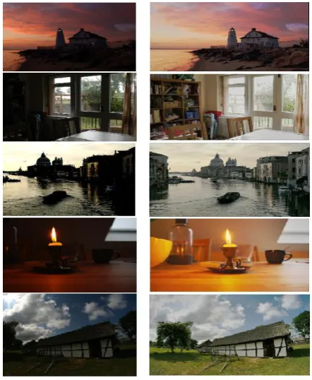
The experimental result is performed and tested on different exposure images. All these images, are collected from different resources such as some images are of indoor and some are outdoor, with or without a lighting fixture. The under exposed as well as overexposed images are created for references. After result analysis, the proposed method is compared to the existing methods on the basis of image quality measure such as FSIM [32]. Figure 3 shows some examples of low contrast images along with underexpose, over exposed and enhanced contrast images that verifies the effectiveness of the proposed algorithm.

Figure 3: A Sequence with Low Contrast and Enhanced Images

3865 IJSTR©2020

algorithm is tested over different images and some of them are illustrated in figure 3. In this sub-section, comparisons with existing work is performed with proposed CNN Adaptive Single Image Gradient Learner (CNN-ASIGL) on a static scene and a dynamic scene, respectively. Table I represents the comparative performance in under exposed as well as over exposed conditions.

Table I: Comparative Performance Evaluation of FSIM and PSNR Values

Techniques

Under Exposure

FSIM

Under Exposure

PSNR

Over Exposure

FSIM

Over Exposure

PSNR Proposed 0.9762 20.178 0.9943 20.2459 Jianrui[10]

(hybrid loss function)

0.934 19.77 0.9354 20.21 Jianrui[10]

(DSSIM loss function)

0.92 18.47 0.93 19.60

Jianrui [10] (MSE loss function)

0.91 19.43 0.92 20.01

Jianrui [10] (l1 loss function)

0.91 18.76 0.92 19.96

6.

CONCLUSION

In many real time image applications, one of the essential step is image enhancement. Many approaches has been used and implemented for image enhancement which totally depends on the type of input image. Out of all image enhancement technique is histogram equalization. Now-a-days multi-histogram equalization is used for equalization as well as enhancement of contrast and brightness of the input images. There are several factors that affect the image quality such as noise, distortion, contrast, exposure, etc. All these factors greatly effect the enhancement techniques. In this paper, the research work is focused on designing of multiple exposure image enhancement technique. For this dataset is taken with different exposure images. For processing, a high quality reference image is generated and used for enhancement of the input low contrast images. Test is also conducted for various input images. The proposed work developed using convolutional neural network (CNN) Adaptive Single Image Gradient Learner. By applying this technique, the input low contrast images are capable to adapt according to high quality enhancement accordingly over-exposed or underexposed input image. The result analysis shows that the developed CNN Adaptive Single Image Gradient Learner significantly outperforms state-of the-art methods, and even outperforms better as compared to existing work. In future work, the proposed work will be extended towards low contrast low resolution images as well as low contrast videos.

REFERENCES

[1]. Singh, P.K., Sangwan, O.P., Sharma, A, ―A Systematic Review on Fault Based Mutation Testing Techniques and Tools for Aspect-J Programs‖, International Advance Computing Conference, IEEE, pp. 1455–1461, 2013.

[2]. Singh, P.K., Panda, R.K., Sangwan, O.P., ―A Critical Analysis on Software Fault Prediction Techniques‖,

World Applied Sciences Journal, Vol. 33, No. 3, pp. 371–379, 2015.

[3]. Singh, P. K., Agarwal, D., Gupta, A., ―A Systematic Review on Software Defect Prediction‖, Computing for Sustainable Global Development, IEEE, pp. 1793– 97, 2015.

[4]. Negi, S.S., Bhandari, Y.S., ―A hybrid approach to Image Enhancement using Contrast Stretching on Image Sharpening and the analysis of various cases arising using histogram‖, Recent Advances and Innovations in Engineering, pp. 1–6, 2014.

[5]. Arunachalam, S., Khairnar, S.M., Desale, B.S., ―Implementation of fast fourier transform and vedic algorithm for image enhancement‖, Applied Mathematics Science, vol 9, issue 45, pp. 2221– 2234, 2015.

[6]. Ramiz, M.A., Quazi, R., ―Design of an efficient image enhancement algorithms using hybrid technique‖, International Journal of Recent Innovative Trends Computer Communication, vol 5, issue 6, pp. 710– 713, 2017.

[7]. Verma, A., Goel, S., Kumar, N., ―Gray level enhancement to emphasize less dynamic region within image using genetic algorithm‖, International conference on Advance Computing Conference, IEEE, pp. 1171–1176, 2013.

[8]. Khan, T.M., Khan, M.A., Kong, Y., ―Fingerprint image enhancement using multi-scale DDFB based diffusion filters and modified Hong filters‖, Optik-International Journal for Light and Electron Optics, Vol. 125, pp. 4206–4214, 2014.

[9]. Shanmugavadivu, P., Balasubramanian, K., ―Particle swarm optimized multi-objective histogram equalization for image enhancement‖, Optics Laser Technology, Vol. 57, pp. 243–251, 2014.

[10]. Jianrui Cai, Shuhang Gu, and Lei Zhang, ―Learning a Deep Single Image Contrast Enhancer from Multi-Exposure Images‖, IEEE Transactions on Image Processing, Vol. 27, No. 4, April 2018.

[11].

https://sites.google.com/site/vonikakis/datasets

http://blog.sina.com.cn/s/blog

a0a06f190101cvon.html

[14].

http://mcl.korea.ac.kr/projects/LDR/LDR

TEST

IMAGES DICM.zip