Classification of Random Boolean Networks
Carlos Gershenson
†,‡†School of Cognitive and Computer Sciences
University of Sussex Brighton, BN1 9QN, U. K. C.Gershenson@ sussex.ac.uk http://www.cogs.sussex.ac.uk/users/carlos
‡
Center Leo Apostel, Vrije Universiteit Brussel Krijgskundestraat 33, B-1160 B russels, Belgium
Abstract
We provide the first classification of different types of Random Boolean Networks (RBNs). We study the differences of RBNs depending on the degree of synchronicity and determinism of their updating scheme. For doing so, we first define three new types of RBNs. We note some similarities and differences between different types of RBNs with the aid of a public software laboratory we developed. Particularly, we find that the point attractors are independent of the updating scheme, and that RBNs are more different depending on their determinism or non-determinism rather than depending on their synchronicity or asynchronicity. We also show a way of mapping non-synchronous deterministic RBNs into synchronous RBNs. Our results are important for justifying the use of specific types of RBNs for modelling natural phenomena.
1. Introduction
Random Bo olean N etworks (R BN s) have been used in diverse areas to mo del co mple x system s. There has been a debate on how suitab le mo dels the y are d epe nding on the ir prop erties, mainly on their updating scheme (Harvey and Bossom aier, 1997; Di Paolo, 2001). Here we make a classification of different types of RB Ns, d epe nding on the ir updating scheme (synchronous, asynchronous, deterministic, non-deterministic), in order to study the p roperties, differences, and similarities of each one of them. The aim of this study is to increase the criteria for judging which types of RBNs are suitable for modelling particular comp lex systems. In the next section we p resent our classification of RB Ns, first mentio ning the prev iously d efined types of RBN s, and then defining three new types of RBNs. In Section 3 we present the resu lts of a series of experiments carried out in a software labo ratory, d evelo ped by us sp ecially for this purpose, and available to the public. Particularly, we present our studies on point attractors, statistics of attractor density in different types o f network, and the homogeneity of RBNs (which valida tes our statistical ana lyses). In Section 4 we propose a (non-optimal but general) method for mapping
deter ministic RBN s into synchronous RBNs. In Section 5 we identify further directions for studying and understanding different types of RBNs. W e conclude estimating the value of our work , and we use our results to clarify a controversy on the proper use of RBN s as models of genetic regulatory networks (Kauffman, 1993; Harvey and B ossomaier, 1997).
2. Random Boolean Networks
There has been no previous classification of different types of RBN s, perhaps because of the novelty of the concept, but there has been enough research to allow us to make a classification of RBNs acco rding to their updating sche mes. Classical Random Boo lean Networks (CRB Ns) were proposed by Stuart K auffma n (19 69) to mo del ge netic regulation in cells. They can be seen as a generalization of (bina ry) cellula r autom ata (CA). T hese were first developed in the late 19 40 's by John von Neum ann (1966), for studying self-replicating mechanisms.
A RB N has n nodes, which have connections (k) between them (n, k 0ù, k#n). The state (zero or one) of a node at time t+1 depends on the states at time t of the nodes which are connected to the node. Here we will limit our study o nly to homogeneo us RB Ns, w here k is the sam e for all no des. L ogic rules (n*2k values in look up tab les) are gener ated r andomly, and they determine how the nodes will affect each other.
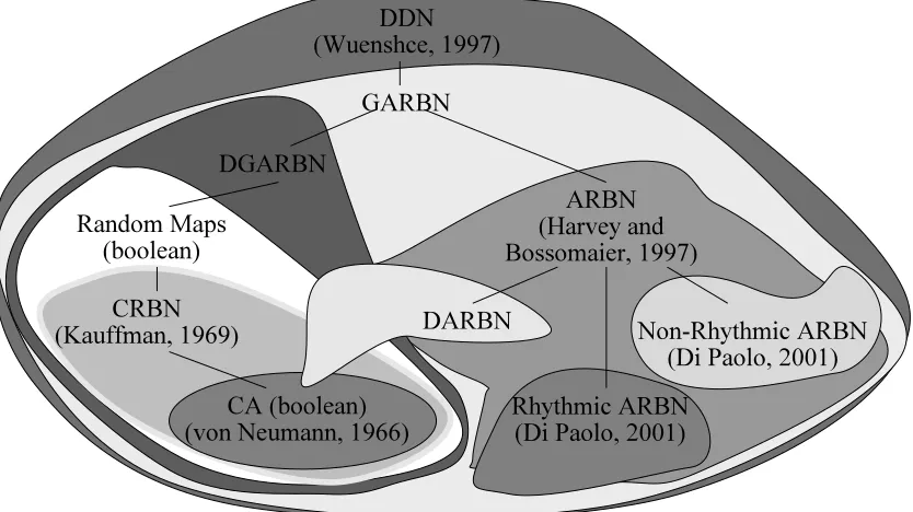
Figure 1. Classification of Random Boolean Networks
CRBNs have attractors, which consist of a state (“point attractor”) or a group of states (“cycle attractor”) which “capture” the dynamics of the network. Since CRBN s are deterministic, once the state of a network reaches an attractor, it will never have states different from the ones in the attractor. And since the number of states of a C RB N is also finite, in theory, an attractor will always be reached.
H arvey and Bo ssomaier (1997) studied Asynchronous Random Bo olean Networks (ARBN s) They have the characteristics of CRB Ns, but their updating is asynchronou s. W ell, in ARB Ns, the upd ating is not only asynchrono us, but also random. Each time step a single node is selected at random in order to be updated. Because of this, in ARBNs there are no cycle attractors (although there are point attractors). The system cannot escape from a point attractor, because no m atter wh ich no de is selected , the state of the network will not change. ARBNs also have “loo se attractors” (Harvey and B osso maier, 199 7), wh ich are parts o f the state space which also capture the dynamics, but since the updating order of the nodes is random, the order of the states will not be repeated deterministically. Although, Di Paolo (2001) evolved successfully ARBNs for finding rhythmic and non-rhythm ic attractors, but ARB Ns with these attractors seem to be a very sm all subset of all possible AR BN s.
In ord er to have a more complete taxonomy of RBNs, we define three types of RBN s, setting all of them and the prev iously expo sed under Discrete Dynamic Networks
(DD Ns), a term introduced by W uensche1 (1997), since we can say that DD Ns have all the pro perties co mmon in a ll types of RBNs: they have discrete time, space, and values. DDNs outside of our scope would b e multivalued netwo rks, but they would be DDN s also. Real-valued networks would not be D DN s, since the ir values are no t discrete, but continuous. Dyna mical System s Th eory stu dies such systems. W e define Deterministic Asynchronous Random Boo lean Networks ( D ARBN s) as ARBNs which do not select at random which node to update. Each node has associated two param eters: p and q (p, q 0ù, q<p), which determine the period of the update (how many time steps the node will wait in order to be updated), and the translation of the update, respe ctively. A node will be updated when the modulus of time t over p is equal to q. If two or more nodes will be updated at a specific time, the first node is updated, and then the second is updated taking into account the new state of the network. T his order is arbitrary, but since there is no restriction in the connection of the nodes by their locality (as with CA ), we ca n have any kind of po ssible D AR BN s with this upd ating scheme . The advantage is that with DARBNs we can model asynchronous phenomena which are not random, a thing which is quite difficult with ARBN s. The refore, DA RB Ns have cycle (and p oint) attractors.
ARBNs have a nothe r limitation : they only u pda te one node at a time. W e define G eneralized A synchronous Random Boolean Netwo rks (GA RB Ns) as ARBNs which can up date
1
any number of nodes, picked at random, at each time step. Th is means that GARBNs can go from not updating any node at a time step, passing to updating only one (as ARBNs), updating some nodes synchronously, to updating all the nodes synchrono usly (as CRBN s). As ARBN s, they are non-deterministic, so again there are no cycle attractors, only point and loose attractors.
As we did with DA RB Ns, we introd uce the para meters p and q asso ciated to each nod e to d efine D eterm inistic Generalized Asynchronous Random Boolean Networks (DGAR BN s). They do not have the arbitrary restriction of DA RB Ns, so if two o r mo re no des a re de termined b y their p’s to be up dated at the sam e time ste p, they w ill be updated synchro nous ly, i.e. they will all be updated at time t+1 taking into account the state of the network at time t. Note that DGARBNs and D AR BN s overlap in the spe cific cases when p and q are such that one and o nly one nod e is updated each time step (fo r exam ple, a network of two nodes (n=2), one being upd ated a t even tim e steps (p= 2, q= 0), and ano ther being updated at uneven time steps (p=2, q=1)).
Also other spec ific configu rations produce the same behaviour for all the typ es of ne twork indep endently of the ir updating schemes (e.g. when k=0, or when all states are point attractors).
Figure 1 shows a graphic representation of the classification just described above.
As we stated, we classify all RBNs under D DN s. The m ost general are GAR BN s, since all the others are particular cases of them. If o n one hand , we ma ke them d eterm inistic with parameters p and q, we will have DGARBN s. Random maps are emerging when n=k, and for all nodes p=1 and q=0. The se ones can simulate with redundancy any CRBN, but not otherwise. Th erefo re, CRBNs can be seen as a subset of random maps. B oolean C A are spe cific cases of CR BN s, where the co nnec tivity is limited by the spatial organization of the nodes. On the other hand, if we limit GARBNs for updating only one node at a time, we will have ARBNs. If we make them deterministic, we will have DAR BN s. There are also special cases of AR BN s with rhythm ic and n on-rhyth mic attractors. Very probab ly GARB Ns with rhythmic and non-rhythm ic attractors can be found. Most types of RBNs can behave in the same way in limit cases (e.g. when k equ als zero, or when the number of attractors equals n).
RBN updating scheme
CRBNs synchronous, deterministic ARBNs asynchronous, non-deterministic DARBNs asynchronous, deterministic
GARBNs semi-synchronous, non-deterministic DGARBNs semi-synchronous, deterministic
Table 1. Updating schemes of RBNs.
Here we will study the properties of CRBNs, ARB Ns, DA RB Ns, GARBNs, and DGARBN s. Table 1 shows the characteristics of the updating schemes for each one of these RB Ns. Note that there are no synchro nous , non-d eterm inistic RB Ns. We say that GA RB Ns a nd D GA RB Ns h ave se mi-synchronous updating because in some cases they can behave synchro nous ly (all nodes upd ated a t once ), and in some cases as asynchronously (only one node is updated at once), but mainly in all the po ssibilities in betwee n, i.e. when some nod es are upd ated syn chro nous ly.
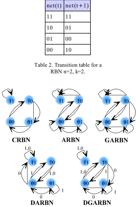
As a simple example, in Table 2 we show the transition table of a RBN of n=2, k=2, p’s={1,2}, and q’s={0,0}. Figure 2 show s the different trajectories that the RBN will have, depending on its updating scheme.
net(t) net(t+1) 11 11 10 01 01 00 00 10
Table 2. Transition table for a RBN n=2, k=2.
Figure 2. Graphs of RBNs with different updating schemes. The arrows with numbers indicate which transition will take place
depending on the modulus of time over two.
3.Experiments and Analysis
W e developed a software laboratory for studying the properties of different types o f RB Ns. It is av ailable online to t h e p u b l i c (J a v a s o u r c e c o d e i n c lu d e d ) a t
http://www.cogs.sussex.ac.uk/users/carlos/rbn. It can be used through a web browser, providing a friendly interface for generating, editing, displaying, saving, and load ing RB Ns, and analysing their pro perties. Th e results p resented in this section are product of experiments carried out in our labo ratory.
3.1. Point Attractors
Our first finding is that the point attractors are the same for any type of RB N. In other w ords, if we find a point attractor in an ARBN, if we change the updating scheme to CRBN (or any other), the point attractor will be the same. This is because a poin t attracto r is given w hen fo r all the no des, the ir rules determine that when they will be updated, they will have the same value. T herefo re, it is not impor tant in which order or how many nodes are updated, since none will produce a change in the state of the network.
W e should note that the ba sins of the poin t attracto rs in most cases are very different for different types of RBNs. The cycle and loose attractors and their basins also change (tough not always) d epe nding on the updating scheme. But for a determined network connectivity and rules, the point attractors will be the same.
3.2. Attractor density
For this section, we obtained with our laboratory statistics from 1000 networks of each of the presented values of n and k. First we generated randomly a RB N with the specified n, k, p, and q, and then we tested the RBN with the different updating schemes. For e ach typ e of ne twork we tested all pos sible initial states, running them for 1 000 0 time steps, expecting to reac h an attracto r. Then we searched for attractors of period smaller than 50 for CRBNs and 200 for the other deterministic cases (checking that the state and periods would be the same as the ones as t=10000), and point a t t r a c t o r s f o r t h e r a n d o m c a s e s ( i f state(10000)=state(10001)=...=state(10050)). For all our experime nts the p’s for all the nodes were generated randomly, taking values between 1 and 4, and all q’s=0.
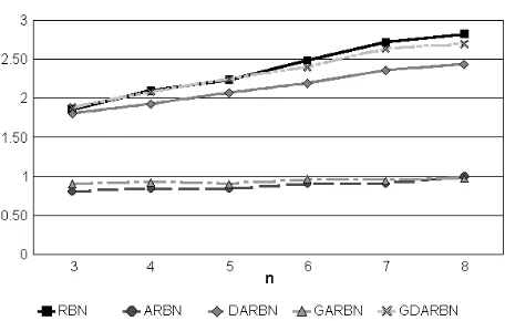
Figure 3 shows the average number of de terministic attractors for networks of n’s between 1 and 5, with all the ir pos sible k’s (from 0 to n). Figure 4 shows the same information for netw orks o f k=3 and n between 3 and 8. Remember that RB Ns which are updated with random schemes (ARB Ns and GA RB Ns) can o nly have deter ministic attractors of period one (point attractors), and if one network has a point attractor, the other types of network will have the
same poin t attractor. We can see from Figure 3 that the average of po int attracto rs in AR BN s is roughly lower for k=3, consistent with results of Harvey an d B ossoma ier (1997)2. From both figures we can see that DARB Ns, and DGARBNs even more, are very close to the number of attractors found in CR BN s. We c an see here that there is a very big difference due to the randomness of the updating, and not so much due to the de gree o f synchro nicity.
W e can also see that, for deterministic RBNs, the growth of the average number o f attracto rs as we increa se n, with constant k, seems to be linear, consistent with the results of Bilke and Sjunnesso n (200 2) for CR BN s.
Figure 3. Average number of deterministic attractors.
Figure 4. Average number of deterministic attractors, k=3.
No te that when there is no connectivity (k=0), there is no interesting updating, since the networks, independ ently of their initial state or updating scheme, will reach a final state.
2
It is because o f this that all RBNs have one and only one point attractor for any value of n when k=0.
W e can appreciate the percentage of states which b elong to an attracto r for the sa me ne twork s in Figure 5 and Figure 6. Here we can see that RBN s have more states in attractors than DGARBNs and DARBNs. This suggests that the average period of the cycle attractors is higher for RB Ns.
Figure 5. Percentage of states in attractors.
Figure 6. Percentage of states in attractors.
W e can also see in Figure 5 that for deterministic RBNs, the number of states in an attractor increases with k. But the percentage of the state s in attractors seems to d ecrease exponentially as n increases for all types of RBN.
W e would also like to know exactly how many states there are in each attractor, not only their perc entage . But w e should note that, even when CRBNs, ARBNs, and GARBNs have 2n pos sible states, this is increased in D ARB Ns and DG ARB Ns, because of the introduction of the updating p eriods. T his is, a network with the same state, may be updated in a different way dep ending on the time it re ache s that state. T herefo re, in DARBNs and DGAR BNs we need to take into account the least com mon multiple of all p’s, an d we will have LCM (pi)* 2n possible states. As we can see, the periods of the attractors in DARBNs and DGARBNs grow in comp arison to CR BN s, but since there are also more states, the ratio between states in attracto rs and total states is e quiva lent. But for calculating the number of states, we normalized the number o f states dividing them b y their total n umb er of state s divid ed b y 2n.
No te that this produces a change only in DARB Ns and DGARBNs (since all other RBNs have 2n states), setting
them in values comparable to the ones in the other R BN s. These results can be seen in Figure 7 and Figure 8.
The values of AR BN s and G ARB Ns are the same as the ones in Figure 3 and Figure 4, since the states in attractors are point attractors. Again we can see that the pe riod of the cyc le attractors are higher for RBNs than for DG ARB Ns, and these are a bit higher than the ones of DA RB Ns. In deter ministic RBN s we can see that the number of states increases with k. They also seem to increase with n, but C RB Ns inc rease this number much faster than the normalized DGA RBN s and DA RB Ns. This increm ent for the deter ministic networks (as we increa se n) ap pea rs to be linear. T he stee pness of this increment seems to be increased with k. But as we have seen, the pe rcenta ge of sta tes in de terministic attractors decreases with n, since the number of states of the network is doubled for each node we add to the network.
Figure 7. States in attractors (relative).
Figure 8. States in attractors (relative).
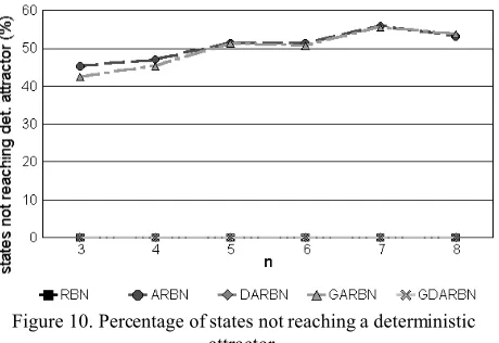
(that is, the states which do reach an attractor ), and of cou rse the size of the basins of attrac tion of the loose attracto rs. It seems, but is not clear, that the percentage of states which do not reach point attractors increases as n does. On the other hand, it is obvious that there is a lower probability to reach a point attractor when point attractors are harder to find (k=3).
Figure 9. Percentage of initial states not reaching a deterministic attractor.
Figure 10. Percentage of states not reaching a deterministic attractor.
From the inform ation gathered in all these charts, we can see that there is a regular order (with very few exception s) on the number of attractors, and states in attractors for the different types of RBNs. CRB Ns are on top, having the highest number of attractors and states in attractors. On the bottom, there are ARBN s, which have the lowest values. In the middle of the rest, there are DARBN s, and the generalized versions are in the spaces left in between, but very close and above DGARBNs of DARBNs and GARBNs of ARB Ns.
The reason of this can be explained with the different updating schemes. RBNs with no n-dete rministic u pda ting will have less deterministic attractors because they can only have point attractors. Anyway, GARBN s have a slightly higher probability than A RB Ns to reach one fa ster since their updating is semi-synchronous, and this shou ld enla rge the ir basins of attraction. Since RB Ns w ith deter ministic updating have cycle attra ctors, this explains why they have more
attractors and states in attractors than non-determ inistic ones. But we can see that the se num bers in creas e from asynchronous to semi-synchronous to synchronous. The lack of synchronicity increases the complexity of the RBN, because we need parameters p and q to make the updating, enhancing the num ber o f possib le states and interactions. And this complexity changes the attractor basins, transforming and enlarging them. This reduces the number of attractors and states in attractors.
3.3. Possible Networks and Statistics
W e saw that for a specific network with homogene ous connectivity, there are n*2k (binar y) values in the rules of the network. Therefore, there are 2n*2^k pos sible ne twork s.
For any fixed n and k, if we change the connectivity, we will have n etworks red unda nt with these 2n*2^k (in the number of attractors, attractor basins, etc.). Thus, if we are not interested in the pa rticular connectivity, but on the general properties of RBNs, we will find “only” 2n*2^k equiv alent networks. To get a broad picture of how fast the number of possible networks grow, Table 3 shows the number of possible netwo rks for small n’s and k’s.
n \ k 0 1 2 3 4 5 6
1 2 4
2 4 16 256 3 8 64 4096 1.68E+07 4 16 256 65536 4.29E+09 1.84E+19 5 32 1024 1048576 1.10E+12 1.21E+24 1.46E+48
6 64 4096 16777216 2.81E+14 7.92E+28 6.28E+57 3.94E+115 7 128 16384 2.68E+08 7.21E+16 5.19E+33 2.70E+67 7.27E+134 8 256 65536 4.29E+09 1.84E+19 3.40E+38 1.16E+77 1.34E+154 9 512 262144 6.87E+10 4.72E+21 2.23E+43 4.97E+86 2.47E+173 101024 1048576 1.10E+12 1.21E+24 1.46E+48 2.14E+96 4.56E+192
Table 3. Possible equivalent networks for n nodes and k connections (2^(n*(2^k))).
As we can see, the number of possible networks grows treme ndo usly fast. So, if we managed a statistical space of only 1000 sample networks, how representative will it be for n=8, k=3, if our sample is roughly 1.84*10-16 of the po ssible networks?
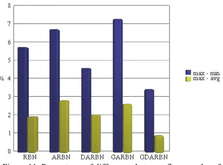
could see (at least for this case) that the farthest we can get from an average value is less than 5%, even when our samples are taking 1.84*10-16 of the poss ible netwo rks. T his means that the glo bal p rop erties of RB Ns a re very uniform. Th is is, it is not that there are no netwo rks with n attractors, but there is only one. There are also very few netwo rks with all their states in an attractor, and there are many networks with the characteristics we extracted in our expe riments. All the values that we extracted in different trials in our experiments also were very close to each other.
Also, since the plots we obtained for attra ctor d ensity (Figures 3-8) fir ve ry well with linear or expo nential curves, it appears that our statistics match the actual a ttractor density without much error. This is not the case for Figures 9-10.
Figure 11. Percentages of differences between five samples of 1000 networks (number of attractors).
4. Mapping Deterministic RBNs to CRBNs
If a RBN is deterministic, we can map it to a CRBN . Of course, this is interesting only if the R BN is a D ARBN or a DGARBN.
Perhaps this is not optimal, but a way of obtaining the same behaviour of a D AR BN or D GA RB N o f specific n, k, p’s, and q’s is to create a CRBN of n+m nodes and k+m connectivity, where 2m$LCM (pi). W e use the least common
multiple of all p’s in ord er to co ntemp late all the p ossible combinations of differe nt nod es be ing up dated , but in sp ecific networks this might be redundant. The m nod es to be added should encode in binary base the time mod ulus LCM(pi).
W hat was a function of time in the DARBN or DGARBN, now is a function in the network. Of cour se there is a redundancy at least wh en in the m nodes encoding time there is a binary value greater than LCM (pi).
In Table 4 we can appreciate the mapping to a CRBN of the DA RB N w ith transition s show n in T able 2 and g raph in Figure 2. Table 5 shows the mapp ing for the case of the respective DG ARB N. The no de m (2m$LCM(pi), LCM (pi)=2,
m=1) which is added is shown in grey. These CR BN s have the same behaviour than the deterministic non-synchronous
networks from Figure 2, but the network itself is more complex (n=3, k=3 ).
It would be too rushed to say that ther efore all deter ministic non-synchronous RBNs can be seen as CRB Ns, since we do not know how redundant the proposed mapping is, and therefore the complexity of the network might be increased too much. It should still be studied how similar are the properties of CRBN s and deter ministic RB Ns m app ed to CRB Ns.
W e can see that the fact that CRBNs have a higher attractor density is related to the fact that DARBNs and DGARBNs are more complex than a CRBN of the same n and k (b ecause of the p’s and q’s). As we have seen in our experiments, the attractor density of RBNs decreases exponentially as we increase n. If we want to map the behaviour of a de terministic non-synchronous RBN to a CRBN, we need to add m nodes (2m$LCM (pi)), and such CRBN would see its attractor
density reduced, just as DARBNs and DG ARBN s have a lower attracto r den sity.
net(t) net(t+1) 111 110
101 000
011 010
001 100
110 111
100 001
010 001
000 111
Table 4. Map of DARBN to CRBN.
net(t) net(t+1) 111 110
101 000
011 010
001 100
110 111
100 011
010 001
000 101
Table 5. Map of DGARBN to CRBN.
5. Unattended Issues
order-complexity-chaos in the types of RBNs defined here also needs to be addressed. The study of non-homogeneous RBNs and hybrid RBN s should also increase our understanding of these mod els. Finally, since cellular autom ata could be seen a s spec ial cases of RB Ns, the results presented here can be applied for understanding the differences caused by the updating schemes of cellular automata.
Bec ause of the computational complexity of RB Ns, it is difficult to study the ir mathe matica l prop erties straig htawa y. W e believe this is a challenge for mathematicians, which could be ad dress ed with the aid of our softwar e laboratory. For example, it would be very useful to find formulae for determining the inform ation w e ob tained statistically for any given n and k, especially for non-d eterm inistic RBN s, where statistics seem to be more evasive. This would also validate or nullify the results presented here.
All these issues should be addressed if we desire to increase our u nderstand ing of RB Ns.
6. Conclusions
In this work we presented the first proposed classification of different types of random boolean networks, depending on the synchronicity and determinism of their updating schem es. W hile doing so, we defined three new types of RB Ns: DA RB Ns, GAR BN s, and DGA RBN s. Using a software laboratory we developed (source code available), we obtained some of the general properties of the different RBN s through statistical analysis, noticing when they have similarities and differences, but further study is req uired to fully understand all the properties o f different RBN s.
CRBNs and ARBNs are different mostly beca use the first ones are d eterm inistic and the second are not, but CRB Ns are not that different to non-synchronous deterministic RBNs. DARBNs are much more similar to C RB Ns than to A RB Ns. W e agree to the critics to synchronou s CRB Ns in the sense that when they are used to mo del an y phen ome na, their synchro nicity needs to be justified somehow. But as we have seen, asynchrono us DA RB Ns are sim ilar to CRB Ns, bec ause both are deterministic, as opposed to ARBNs. Of course, while modelling, the choice for deterministic or non-deterministic RBNs should be also justified.
Par ticularly, Stuart Kauffman’s work (1993) was criticized (Harvey and B ossomaier, 1997) because it assumed that gene tic regulatory networks were synchronic. W e agre e with the critic that the synchronicity was an assumption withou t a base, but we do not believe that genetic regulatory networks are random. They should be most probably modelled better with DARB Ns, if we can model the updating periods for each gene. But one of the main results of Kauffman was that the number of attractors on CRB Ns could explain why there are very few cell typ es in comparison with all the possible initial states of their genes. Since the number of attrac tors in
DARBNs is very close to the ones in CRBNs (and the number in DG AR BN s is much closer , since they are semi-synchronic), we can say that this particular result, still holds (perhaps with minor adjustments), since the number of attractors does not depend too much in the synchronicity of the updates, as they depend on their determinism.
Acknowledgements
I appreciate the valuable comments and suggestions received from Inman Harvey, Ezequiel Di Paolo, Andrew W uensche, and two anonymous referees. This work was supported in part by the Consejo Nacional de Ciencia y Tecnolo gía (CONACYT ) of México and by the School of Co gnitive and Computer Sciences of the University of Sussex.
References
Aldana, M., S. Copp ersmith and L. P. Kadanoff (2002). Bo olean D ynamics with Ran dom Coup lings.
Bilke, S. and F. Sjunnesson (2002). Stability of the Kauffman M ode l, Physical Review E 65 016129.
Di Paolo, E. A. (200 1) R hythmic and N on-rhyth mic Attractors in Asynchrono us Rand om B oolean N etworks. Biosystems, 59 (3 ), pp. 1 85-1 95.
Ha rvey, I. and T . Bo ssom aier (1 997 ) Tim e Out of Jo int: Attractors in Asynchronous Random B oolean Networks. In Proceedings of the Fourth European Conference on Artificial Life (ECAL 97), P. Husband s and I. Harvey (Eds.). MIT Press 1997, pp. 67-75.
Kauffman, S. A. (1969) Metabolic Stability and Epigenesis in Ran dom ly Con structed G enetic N ets. Journal of Theoretical Biology, 22, pp. 437-467.
Kauffman, S. A. (1993) The Origins of Order. Oxford University Press.
von Neumann, J. (1966 ) The Theory of Self-Reproducing Au tom ata. (edited by A. W . Burks), University of Illinois Press.
W uensche, A. (1997) Attractor Basins of D iscrete Netwo rks, D. P hil Th esis, CSRP 4 61, University of Sussex.