Towards a Bayesian Framework for Optical Tomography

Towards a Bayesian Framework for Optical Tomography

Ivo W. Kwee

Thesis subm itted for the degree o f D octor o f Philosophy (Ph.D.) at the U niversity of London.

D epartm ent of M edical Physics and B ioengineering. U niversity College London.

ProQuest Number: U642583

All rights reserved

INFORMATION TO ALL USERS

The quality of this reproduction is dependent upon the quality of the copy submitted.

In the unlikely event that the author did not send a complete manuscript and there are missing pages, these will be noted. Also, if material had to be removed,

a note will indicate the deletion.

uest.

ProQuest U642583

Published by ProQuest LLC(2015). Copyright of the Dissertation is held by the Author.

All rights reserved.

This work is protected against unauthorized copying under Title 17, United States Code. Microform Edition © ProQuest LLC.

ProQuest LLC

789 East Eisenhower Parkway P.O. Box 1346

A

b s t r a c t

Maximum likelihood (ML) is a well established method for general parameter estimation. How­ ever in its original formulation, ML applied to the image reconstruction problem in Optical To­ mography has two serious inadequacies. One is that ML is incapable of distinguishing noise in the data, leading to spurious artifact in the image. The other drawback is that ML does not provide a way to include any prior information about the object that might be available. Noise régularisation is a major concern in imaging and ill-posed inverse problems in general.

The aim of this research is to improve the existing imaging algorithm for Optical Tomography. In this thesis we have taken two approaches to the problem. In the first approach we introduce a

full maximum likelihood (FML) method which estimates the noise level concurrently. We show that FML in combination with a proposed method of hold-out validation is able to determine a nearly optimal estimate without overfitting to the noise in the data.

In the second approach, we will propose a Bayesian method that uses the so-called normal- Wishart density as a parametric prior. We will show that for low degrees of freedom this choice of prior has robust imaging properties and that in some cases the prior can even increase the image resolution (compared to the ML image) but still retain good suppression of noise. We show how

graphical modelling can assist in building complex probabilistic models and give examples for the implementation using a developed C4-+ library.

A

c k n o w l e d g e m e n t s

I am particularly indebted to my supervisors, Prof. David Delpy and Dr. Simon Arridge. They both have guided and encouraged me throughout this work in their own ways.

The Department is truly a first class institute and I must thank all the people who have helped me directly or indirectly. In particular I thank Dr. Martin Schweiger for sharing his knowledge on the FEM and TOAST, Elizabeth Hillman who provided the experimental data and Florian Schmidt for his advice on the instrumentation.

I am very grateful to Dr. Yukio Yamada who introduced me to this field, for enabling my stay in Japan, for his personal guidance and patience.

Thanks also go to Prof. A. P. Dawid without whose lecture and helpful discussions I would not have gained my current level of understanding of Bayesian methods.

C

o n t e n t s

Acknowledgements

4

Preface

9

Symbols

15

1 Introduction to Optical Tomography

33

1.1 Introduction... 33

1.2 Optical Tomography: Imaging with lig h t... 34

1.3 Target Applications of Optical T om og raph y... 38

1.4 Other Functional Imaging T ec h n iq u es... 40

1.5 Optical Tomography as a Nonlinear Ill-posed Inverse P r o b le m ... 42

1.6 Additional References ... 44

2 Photon Migration in Tissues

46

2.2 Absorption and Scattering of Light in T issue... 53

2.3 Photon Transport Models in Highly Scattering M e d ia ... 56

2.4 Boundary and source c o n d itio n s ... 60

2.5 Summary and R eferences... 63

3 Computations Using FEM

65

3.2 Forward Data Computation Using F E M ... 68

3.3 Jacobian and PMDF Computations Using F E M ... 75

3.4 Direct Computation of the Gradient Using F E M ... 80

3.5 Other Solution M ethods... 84

CONTENTS 6

3.5.1 Analytic solutions using Green’s functions ... 84

3.5.2 Numerical solution using the Monte Carlo m e t h o d ... 86

3.5.3 Numerical solution using the finite-differences m e th o d ... 87

3.6 Summary and References... 87

4 Least Squares Estimation

89

4.2 About the Test Reconstructions... 93

4.3 Test R e s u lts ... 97

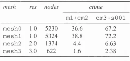
4.3.1 Sensitivity to mesh resolution... 97

4.3.2 Inverse crime examples... 102

4.3.3 Influence of error norm and parameter scaling...103

4.3.4 Sensitivity to source-detector positions...107

4.3.5 Sensitivity to initial guess... 109

4.3.6 Dependence on the number of measurements... I l l 4.3.7 Uncertainty in the geometry...113

4.3.8 Effects of the skin/skull l a y e r . ... 118

4.3.9 Dependence on data noise...120

4.3.10 Dependence on iterations... 124

4.4 Discussion and Additional R e m a r k s ... 129

4.5 Summary and R eferences... 133

5 Full Maximum Likelihood

136

5.2 Optimisation Using I C M ...141

5.3 Convergence Analysis of D a t a ... 145

5.4 Convergence Analysis of S o lu tio n ... 147

5.5 On the log-determinant t e r m ...151

5.6 Chapter S um m ary... 152

6 A Generalised Hold-Out Validation Scheme

153

CONTENTS 1

6.3 Implementation in Gradient-Based Optimisation... 157

6.4 Analysis of Data C onv ergen ce...160

6.5 Analysis of Image Convergence ... 162

6.6 Discussion and Additional R e m a r k s ... 171

6.7 Chapter S um m ary...174

7

Bayesian Regularised Imaging

176

7.2 A Bayesian Framework for Optical Tomography... 183

7.3 Finding Posterior Modes... 194

7.4 Characterisation of the Normal-Wishart P r i o r ... 195

7.5 Régularisation Using Zeroth-Order Priors (Type I ) ...202

7.6 Régularisation Using First-Order Priors (Type I I ) ...208

7.7 Discussion and Additional R e m a r k s ...219

7.8 Summary and R eferences... 221

8

A Hierarchical Mixed Prior Model

223

8.2 Mixed Type-I/Type-II P r i o r s ... 226

8.3 Probability M o d e l...226

8.4 Graphical Model and C-n- Implementation... 228

8.5 Example I: Reconstructions of the Head-Shaped P hantom ...229

8.6 Example II: Reconstructions from Experimental D a t a ... 233

8.7 General Discussion and R em arks...241

8.8 S u m m a r y ... 248

A Derivation of the Boltzmann Transport Equation

250

B

Derivation of the Diffusion Equation

254

C Some Algebra and Probabihty Theory

257

CONTENTS 8

C.3 Some Standard Functions and D istrib u tio n s... 266

D Graphical Modelling in C++

275

D.2 Optimisation of Param eters... 278

D.3 C++ Code Examples Using B eTO A ST... 279

D.4 Summary of classes in the BeTOAST library...284

Afterword

288

Bibliography

289

PREFACE

Introduction to this Thesis

Background. Premature babies have an increased risk of brain damage and it is highly desirable to have an instrument that can continuously monitor the sufficiency of oxygenation in the baby brain. Here at University College London, we have developed an imaging system that uses near- infrared light to probe the neonatal head and visualises the distribution of oxygenated blood in the interior.

Light travelling through biological tissue is strongly attenuated and suffers heavily from scat­ tering which severly hampers the image reconstruction. The image reconstruction problem in Optical Tomography is mathematically said to be severely ill-posed, which generally leads to a highly blurred or noisy image. It is known that additional prior information may greatly enhance the image.

Aims. The work described in this thesis is aimed at improving the imaging reconstruction algo­ rithm. The approach taken comprised two steps,

• Investigation of the limiting factors of the current imaging methods,

• Development of an improved algorithm.

A further aim of this study is to explore the ways in which Bayesian methods can be used in Optical Tomography and the ill-posed problem in general. Inevitably, in taking such a broad approach this has in some circumstances led to a trade off between depth and generality.

CONTENTS 10

To the reader

The ‘classical’ and ‘Bayesian’ method. When I will refer to the ‘Bayesian method’, I do not mean merely the use of priors, but with the ‘Bayesian method’ I mean the whole framework of parameter estimation that is based on probability densities including prior densities. I would rather prefer to use a more descriptive name for the method, such as probabilistic inference, density estimation or probabilistic inverse methods. However, the use of the ‘Bayesian method’ is more common.

Also, when I speak about ‘classical methods’, I do not mean to say that these methods are ‘out­ dated’ in any way. It is common in Bayesian literature to refer to methods that use point-estimates and are based on the maximum likelihood principle as ‘classical’. Neither I am suggesting that the Bayesian method is ‘modem’; maybe the recent computational methods are but Bayes’s theorem dates back to 1763.

To classicists. I hope that this thesis may show you the limitations of maximum likelihood (ML) estimation applied to the imaging problem in Optical Tomography. We do not claim that maxi­ mum likelihood is wrong in any way but hope to point out how Bayesian methods can elegantly provide ways to cope with the inadeqacies of ML. In a way the thesis is written from a classical point of view in that we introduce the Bayesian methods not as alternative but as a natural gener­ alisation of classical methods. I will always point out the similarities of our Bayesian models to classical models.

To Bayesians. For Bayesian readers, this thesis describes an interesting application of Bayesian inference to the image reconstruction problem. The inference task in Optical Tomography is special because we are dealing with a problem of high dimensionality, typically involving several 10,000’s of continuous random variables. All densities are multivariate and the diffusion equation renders the problem highly nonlinear so that standard analytic techniques are not applicable; computations have to be done numerically.

A major point is the use of the normal-Wishart as prior density. We show the generality and robustness of such a prior and we show that correct choice of the degrees o f freedom parameter is crucial to obtain the desired behaviour of the prior for imaging purposes.

CONTENTS 11 We will show that conventional gradient-based optimisation may be used for propagation of the graph to retrieve the modal estimates. We give implementations in C++ of our Bayesian models.

To both. The field of Optical Tomography is an intriguing one, because in my view it is neither well solved by classical methods nor it can be easily tackled by standard Bayesian methods. What I mean to say is that the ill-posed problem (which can be seen as a kind of noisy missing data problem) causes problems when estimating using maximum likelihood, and on the other hand the nonlinearity, the huge problem dimensions, the scarcity of the data and the lack of any clear priors make the Bayesian inference problem still not trivial. I find that Optical Tomography is in a unique position to combine both methods.

This work is by no means suggesting that the Bayesian method is ‘better’. In fact our final conclusion will be to always present both classical and Bayesian solutions together. However, in our opinion we think that the Bayesian way provides a more satisfactory framework for parameter estimation and that to our knowledge it is the only framework that is able to include subjective information in a systematic way.

Overview of Chapters

The order of the chapters follows grossly the course of steps during this research that have taken me from classical estimation to using Bayesian methods. Neither a comparison nor a full appreci­ ation of the Bayesian method could have been done without the chapters on maximum likelihood (ML) estimation. The latters chapters have become rather lengthier than intended, but we needed to investigate what ML estimation can achieve at its best. For the same reason the chapters on Bayesian methods have probably become shorter than we originally intended to cover in all our early ambitions.

CONTENTS 12

Chapter 1, 2 and 3. In Chapter 1 we give an introduction to Optical Tomography, near-infrared spectroscopy, other functional imaging modalities. Chapter 2 presents the physical theory of light propagation in highly scattering media. We discuss general scattering theory, and derive the Boltzmann Transport Equation and the Diffusion Equation. In Chapter 3 we give a mathematical formulation of the so-called forward problem and derive the necessary imaging operators. This chapter introduces the finite element method (FEM) as the basis for our computations. The adjoint operator necessary for gradient calculation of error functions is also derived.

Chapter 4 introduces maximum likelihood (ML) estimation applied to the imaging problem in Optical Tomograhpy. We give an extensive investigation of the sources of random imaging errors including Gaussian noise, source and detector position errors, uncertainties in geometry, FEM mesh resolution and sensitivity of the ML estimate to the initial guess. The conclusion will be that the ML image is too sensitive to these random errors and naive estimation fails due to the noise if no régularisation or early stopping is applied to the iterative scheme.

In Chapter 5 and 6 we propose so-called full maximum likelihood (FML) and a hold-out vali­ dation technique. These methods extend the ML framework in two ways. First, we show that by including the covariance matrix in the estimation FML shows improved convergence as compared to naive ML, and moreover FML can succesfully estimate the level of noise in the data. We use an iterative-conditional-mode (ICM) method for the optimisation.

Secondly, we propose an online validation method by validating the GML estimates during the reconstruction using a random selection of half of the original data. By monitoring the solution norms we show that validated GML is able to (almost) optimally stop the iterative reconstruction before noise contaminates the image.

CONTENTS 13 from simulated data. We also introduce graphical modelling and our C++ library that can easily implement the probabilistic models that are described.

Chapter 8 is the final chapter in which we extend the basic Bayesian model as described in the previous chapter with an additional level of priors (hyperpriors) and allow mixed Tikhonov-type and Markov-type priors at a single level. We demonstrate this model using both simulated and

real data obtained from experiments.

L

i s t

o f

S

y m b o l s

General Notation

Vectors are written in lower case bold typeface, e.g. x . Matrices are written in upper case bold typeface, e.g. A . Operators are written using calligraphic style, e.g. T . Units of length are in millimetres, if not specified otherwise.

Below is a list of symbols summarised for each Chapter. Some symbols may have been rede­ fined in different Chapters. The symbols are approximately ordered in order of first appearance.

Chapter 1: Introduction

symbol definition name

NIR near-infrared

OT Optical Tomography

y general data vector

6 general image vector

V general projection operator

Chapter 2: Photon Migration in Tissues

symbol definition name

DE diffusion equation

NIR near-infrared

FEM finite elements method

TE transport equation

TPSF temporal point spread function

E electrical field

CONTENTS 15

Jfl Bessel function of order n

Hn Hankel function of first kind of order n

A wave length

e

CTa absorption cross section

o-g scatter cross section

Mo absorption coefficient

Ms scattering coefficient

Ms (1 ~ m)ms reduced scattering coefficient

Mt linear attenuation coefficient

$ radiant intensity

fi angular direction variable

(t> photon density (or fluence)

p ( f i , f i ' ) scatter phase function from direction f i into direction f i'

Q photon source

J — photon flux

I intensity

9 anisotropy parameter

K (photon) diffusion coefficient

S surface

fi solid angle

A reflection parameter

( measurement position

r exitance

fi outward normal vector

G Green’s function

w frequency

Chapter 3: Computation Using the Finite-EIement Method

CONTENTS 16 FEM PMDF TPSF

y

e

y

ya

(i">

J

v e

photon measurement density function temporal point spread function general data vector

general image vector projection operator

calculated projection vector photon density

2 th nodal solution coefficient domain

position time

speed of light diffusion coefficient absorption coefficient boundary parameter frequency

integrated intensity exitance

nth temporal moment nth Melllin factor nth central moment

Normalised Laplace transform with parameter s

CONTENTS 17

M measurement matrix

Qj partial gradient of the jth source

Chapter 4: Maximum Likelihood Reconstructions

symbol definition name

fi{r) absorption image (function)

n (r) scattering image (function)

N dimension of a single image

/J, absorption image

K scattering image

0 { ^ ,k} combined absorption and scattering image

y data vector

y VO calculated projection vector

yj jth data element

V projection operator

Vj projection operator at jth data point

M j measurement operator at jth data point

V diffusion operator

M total dimension of data

Q error function

Qk error component for kth data type

ak normalisation factor for kth. data type

Mk subdimension of kth data type

m l mean time data type

cm2 variance data type

cm3 skew data type

CONTENTS 18

Chapter 5: Full Maximum Likelihood

Chapter 6: A Generalised Hold-Out Validation Scheme

symbol definition name

ML maximum likelihood

FML full maximum likelihood

ICM iterative conditional mode

Q error function

6 {a*? combined absorption and scattering image

y data vector

S data covariance matrix

V projection operator

S sample covariance matrix

S sample variance (scalar)

M dimension of full data

K number of data types

(7 standard deviation

ak covariance scaling factor kth data type

C k fixed covariance A:tb data type

r split ratio

Chapter 7: Bayesian Regularised Imaging

Chapter 8: A Hierarchical Mixed Prior Model

symbol definition name

GPU great prior uncertainty

p general probability density

7T prior density

fif normal (or Gaussian) density

W Wishart density

CONTENTS

Q Gamma density

V degrees of freedom

\ number of measurement parameter

$ precision matrix

K

S

y

absorption image (vector)

K, scattering image (vector)

V projection operator

E hypothesis

data precision

Q error function

K number of data types

M dimension of a single data type

L

i s t

o f

F

i g u r e s

1.1 Artist’s impression of Optical Tomography... 34

2.1 Graphical representation of broadening of a picosecond pulse propagating through a highly scattering medium... 46 2.2 Example of a density plot of the total scattered field computed by Mie theory. . . 51 2.3 Absorption spectrum of oxyhaemoglobin and deoxyhaemoglobin... 55

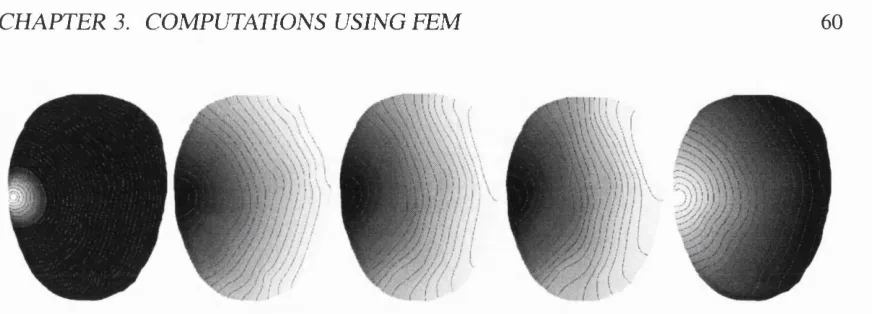
3.1 Examples of FEM solutions for, from left to right, integrated-intensity (log-scale), mean time, variance, skew and Laplace (s=0.001) data types... 69 3.2 Graphical representation of time-integral transformations of the T P S F ... 71 3.3 Example of an absorption PMDF for integrated intensity through a layered

head-model... 76

4.1 Head phantom with outlines of the defined regions... 95 4.2 Enlarged view of meshes with different resolution... 97 4.3 Reconstructed images of a homogeneous object using cm 3 + s00 1 data created

from meshO but reconstructed on other meshes... 99 4.4 Same as Figure 4.3 but for ml+cm2 data... 99 4.5 Absorption images of the head-shaped phantom for different mesh resolutions

using simulated cm3 + s 0 01 data created from m eshO ... 101 4.6 Same as Figure 4.5 but for ml+cm2 data... 101 4.7 Scattering images of the head-shaped phantom for different mesh resolutions us­

ing simulated cm 3+s 0 01 data created from m eshO ...101 4.8 Same as Figure 4.7 for ml+cm2 data... 101 4.9 “Inverse crime” images of absorption coefficient for different mesh resolutions

using cm3+s 0 01 data...103 4.10 Same as Figure 4.9 but for ml+cm2 data...103

L IS T OF FIGURES 21

4.11 “Inverse crime” images of scattering coefficient for different mesh resolutions using s001+cm 3 data... 103 4.12 Same as Figure 4.11 but for m l+cm2 data...104 4.13 Solution errors for (/ia, «) for different combinations of error norm and parameter

rescaling...105 4.14 Residual data error trajectories for different combinations of error norm and pa­

rameter rescaling... 105 4.15 Reconstructed absorption images using cm 3+s 0 01 data types for different com­

binations of error norm and parameter rescaling...106 4.16 Same as Figure 4.15 but for ml+cm2 data... 106 4.17 Reconstructed scattering images for different combinations of error norm and

parameter rescaling using cm3+s 0 01 data types... 106 4.18 Same as Figure 4.17 but for ml+cm2 data... 106 4.19 Absorption reconstructions with perturbed source-detector positions from cm 3+s 0 01

data on m e sh 2 ...107 4.20 Same as Figure 4.19 but for ml+cm2 data types... 108 4.21 Scattering reconstruction with perturbed source-detector positions from cm3+s 0 01

data on m e sh 2 ...108 4.22 Same as Figure 4.21 but for ml+cm2 data... 108 4.23 Reconstructed absorption images (left) and scattering images (right) for different

initial values... 110 4.24 Same as Figure 4.23, but for ml+cm2 data...I l l 4.25 Reconstructed absorption images using cm 3+s 0 01 data types for different num­

ber of measurements... 112 4.26 Same as Figure 4.25 but for ml+cm2 data...112 4.27 Reconstructed scattering images using cm 3+ s001 data types for different num­

ber of measurements... 113 4.28 Same as Figure 4.27 but for m l+cm2 data types... 113 4.29 Absorption (left) and scattering (right) images on scaled meshes using cm 3+s 0 01

L IST OF FIGURES 22 4.30 Optimal absorption images (left) and scattering images (right) on scaled meshes

using cm3+s 0 01 data types...116 4.31 Absorption (left) and scattering (right) images on scaled meshes using m l+cm2

datatypes...116 4.32 Optimal absorption (left) and scattering (right) images on scaled meshes using

m l+cm2 data types...117 4.33 images with skin/skull boundary using c m 3 + s0 01 data types 119 4.34 Scattering images with skin/skull boundary using cm3 + s 0 01 data types...119 4.35 Absorption images. Same as Figure 4.33 but for ml+cm2 data types... 119 4.36 Scattering images. Same as Figure 4.34 but for m l+cm2 data types...120 4.37 Absorption and scattering images of a homogeneous object from noisy data using

cm 3+ s001 data for (1+1)%, (3+3)%, and (10+10)% noise...122 4.38 Same as Figure 4.37 but for ml+cm2 data... 122 4.39 Absorption images from noisy data using a combination of cm 3 + s0 01 data-types. 123 4.40 Scattering images from noisy data using a combination of cm 3+ s001 data-types. 123 4.41 Absorption images. Same as Figure 4.39 but for m l+cm2 data-types... 123 4.42 Scattering images. Same as Figure 4.40 but for ml+cm2 data-types...124 4.43 Absorption images of iteration 1, 2, 4, 10, 20 and 60 of reconstruction from noisy

data using cm 3+s 0 01 data types with (3+3)% noise... 125 4.44 Left to right: Target, and scattering images of iteration 1 ,2 ,4 , 10, 20 and 60 of

reconstruction from noisy data using cm 3+s 0 01 data types with (3+3)% noise. . 125 4.45 Residual trajectories for cm 3+ s001 (left) and m l+cm2 (right) for various com­

binations of noise... 126 4.46 Absorption (left) and scattering (right) solution norm trajectories of various comib-

inations of noise using cm3+s 0 01 data-types...126 4.47 “Best” absorption images from noisy data using cm 3+s 0 01 data-types...127 4.48 “Best” scattering images from noisy data using a combination of cm 3+ s001

data-types...127 4.49 Left to right: target, absorption images of iteration 1, 2, 4, 10, 20 and 60 of

L IS T OF FIGURES 23

4.50 Left to right: target, scattering images of iteration 1, 2 ,4 ,1 0 , 20 and 60 of recon­ struction from noisy data using ml+cm2 data types with (3+3)% noise... 127 4.51 Absorption (left) and scattering (right) solution norm trajectories of various comib-

inations of noise using m l+cm2 data-types...128 4.52 “Best” absorption images from noisy data using m l+cm2 data-types... 128 4.53 “Best” scattering images from noisy data using a combination of m l+cm2 data­

types... 128 4.54 Illustration of a frequency domain system...132

5.1 Typical error terms for fixed (using WLS; prefixed ‘f ’) and dynamically estimated covariance (using FML; prefixed ‘d’)...145 5.2 Typical error terms for fixed (using WLS; prefixed ‘f ’) and dynamically estimated

covariance (using FML, prefixed ‘d’)...146 5.3 Solution norms for absorption (left) and scattering image (right) from noisy cm 3+s 0 01

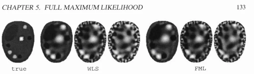
data for reconstructions using WLS with fixed covariance (prefixed “f ’) and FML with dynamically estimated covariance (prefixed “d”)... 149 5.4 Reconstructed absorption images from cm 3+ s001 data using WLS with fixed

or FML with dynamically estimated covariance at various combinations of noise levels... 149 5.5 Reconstructed scattering images from cm 3+ s001 data u s i n g o r dynami­

cally estimated covariance at various combinations of noise levels...149 5.6 Solution norms for absorption (left) and scattering images (right) from noisy

m l+cm2 data for reconstructions usmg fixed covariance (prefixed “f ’) and dy­ namically estimated covariance (prefixed “d”)...150 5.7 Reconstructed absorption images from m l+cm2 data using ML with fixed and

FML with dynamically estimated covariance at various combinations of noise levels... 150 5.8 Reconstructed scattering images from m l+cm2 data using ML with fixed and

L IS T O F H G U R E S 24 6.1 Illustration of hold-out validation to avoid overfitting. The black dots are data

points used for estimation... 157 6.2 Trajectories for error terms for validated generalised maximum likelihood (VFML)

and not validated FML (FML)...161 6.3 Solution norms for absorption (left) and scattering (right) images from citiB+s 0 01

data with (34-10)% noise for split ratio of 0, 1, 10, 25, 50 and 80%...163 6.4 Absorption images from cm34-s001 data with (34-10)% noise for various split

ratio... 163 6.5 Scattering images from cm3 4-s0 01 data with (34-10)% noise for various split ratio. 164 6.6 Solution norms for absorption (left) and scattering (right) images from m l 4-cm2

data with (34-10)% noise for split ratio 0, 1,10, 25, 50 and 80%... 164 6.7 Absorption images from m l 4-cm2 data with (34-10)% noise for various split ratio. 164 6.8 Scattering images from ml4-cm2 data with (34-10)% noise for various split ratio. 165 6.9 Solution norms for absorption (left) and scattering (right) images from cm3 4-s 0 01

data with (34-10)% noise u s i n g o r reselected (prefixed ‘r ’) validation points for a split ratio of 1, 10, and 50%... 165 6.10 Absorption images from cm34-s001 data with (34-10)% noise u s i n g o r res­

elected validation points...166 6.11 Scattering images from cm3 4-s 0 01 data with (34-10)% noise using fixed or rese­

lected validation points...166 6.12 Solution norms for absorption (left) and scattering (right) images from m l 4-cm2

data with (34-10)% noise using fixed or reselected (prefixed ‘r’) validation points for a split ratio of 1, 10, and 50%... 166 6.13 Absorption images from ml4-cm2 data with (34-10)% noise u s i n g o r rese­

lected validation points...167 6.14 Scattering images from m l 4-cm2 data with (34-10)% noise using or rese­

lected validation points...167 6.15 Solution norms for absorption (left) and scattering images (right) from cm3 4-s 0 01

L IS T OF FIGURES 25

6.16 Absorption images from cm 3+s 0 01 data with (3+10)% noise for non-scaled and scaled validation e r r o r . ... 169 6.17 Scattering images from cm 3+ s001 data with (3+10)% noise for non-scaled and

scaled validation e r r o r . ... 169 6.18 Solution norms for absorption (left) and scattering images (right) from ml+cm2

data with (3+10)% noise using non-scaled (no prefix) and scaled (prefixed “s”) validation error for split ratio 1,10 and 25%...170 6.19 Absorption images from ml+cm2 data with (3+10)% noise for non-scaled and

scaled validation e r r o r . ... 170 6.20 Scattering images from m l+cm2 data with (3+10)% noise for non-scaled and

scaled validation error. ... 170

7.1 Illustration of Bayes’ theorem. The prior density is multiplied with the likelihood to obtain the posterior density... 178 7.2 Graphical model corresponding to the Bayesian model estimation of a dual pa­

rameter and dual data type problem... 192 7.3 Graphical model corresponding to our Bayesian model showing densities explicitly. 193 7.4 Plot of one-dimensional normal-Wishart log-density as function of 6 with K =

(1 + g) for different different values of ç = 0, 1,4 and 40... 199 7.5 Absorption images from noiseless simulated cm 3+ s001 data using a Type-I

normal-Wishart prior for values of q and prior precision 0o- Lower left image: target object...203 7.6 Scattering images from noiseless simulated cm3+s 0 01 data using a Type-I normal-

Wishart prior for values of q and prior precision 0o- Lower left image: target object. 204 7.7 Solution norms of absorption (left) and scattering images (right) from noiseless

simulated cm 3+ s001 data using a Type-I normal-Wishart prior for values of q

and different prior precision... 205 7.8 Absorption images from simulated noisy cm 3+s 0 01 data using a Type-I

normal-Wishart prior for values of q and prior precision <f)Q. Lower left image: target object... 206 7.9 Scattering images from simulated noisy cm2 + s 0 01 data using a Type-I normal-

L IST OF FIGURES 26 7.10 Solution norms of absorption (left) and scattering images (right) from simulated

noisy cm 3+ s001 data using a Type-I normal-Wishart prior for values of q and prior precision... 208 7.11 Graphical model corresponding to the Bayesian model with Type-II normal-Wishart

priors...212 7.12 Absorption images from noiseless data using a T^pe-II normal-Wishart prior for

values of q and prior precision ^o- Lower left image: target object...213 7.13 Scattering images from noiseless data using a Type-II normal-Wishart prior for

values of q and prior precision ^o- Lower left image: target object...214 7.14 Solution norms of absorption (left) and scattering images (right) from cm3+ s 0 01

corresponding to the images in Figure 7.12 and Figure 7.13...215 7.15 Absorption images from noisy data using a Type-II normal-Wishart prior for var­

ious degrees of freedom and prior precision. Lower left image: target object. . . . 216 7.16 Scattering images from noisy data using a Type-II normal-Wishart prior for vari­

ous degrees of freedom and prior precision. Lower left image: target object. . . . 217 7.17 Solution norms of absorption and scattering images from noisy cm 3+s 0 01 using

Type-II normal-Wishart p r io r ... 218

8.1 Graphical model of the hierarchical mixed prior model... 229 8.2 Graphical model of the hierarchical mixed prior model showing densities explicitly. 230 8.3 Images of the head-shaped phantom using the hierarchical mixed prior model . . 233 8.4 Photograph of experimental setup of the ‘basic’ phantom (courtesy of F.E.W.

Schmidt)... 234 8.5 Comparison of absorption images of the ‘basic’ phantom using ML and Bayesian

methods... 236 8.6 Same as 8.5 but using a logarithmic scale for the grey values... 237 8.7 Comparison of scattering images of the ‘basic’ phantom from experimental m l+cm2

data using ML and Bayesian methods... 237 8.8 Same as 8.7 but using a logarithmic scale for the grey values... 237 8.9 Recovered values for absorption and reduced scattering coefficient for rods A, B

L IS T OF FIGURES 27 8.10 Recovered values for the standard deviation of data for the Bayesian image I and

Bayesian image I I ...239 8.11 Values of the estimated prior mean of absorption (left) and scattering (right) im­

ages for Bayesian image I and Bayesian image II 239

L

i s t

o f

T

a b l e s

1.1 Comparison of different modalities for functional imaging... 41

2.1 Optical properties of human brain tissue at SOOnm... 57

4.1 Values of optical properties of the inhomogeneties in the head-shaped phantom. . 96 4.2 Meshes, resolution (in mm), number of nodes and computation time (in seconds)

for 32 X 32 source-detector pairs... 98 4.3 Relative difference of FEM forward data for homogeneous mesh... 98 4.4 Statistics of estimate of a homogeneous object... 100 4.5 Same as Fig. 4.4 but for m l+cm2 data types...100 4.6 Relative difference of FEM forward data for head mesh...100 4.7 Solution norms for different combinations of scale options...104 4.8 Mean relative difference (in %) of the forward simulated data for different values

for random errors in source/detector positions... 108 4.9 Solution norms for the head-shaped object for different number of source/detectors. 112 4.10 Mean absorption coefficients of head-shaped phantom using cmS+s 0 01 data types. 114 4.11 Mean scattering coefficients of head-shaped phantom using cm3+s 0 01 data types. 114 4.12 Mean absorption coefficients of head-shaped phantom using m l+cm2 data types. 115 4.13 Mean scattering coefficients of head-shaped phantom using m l+cm2 data types. 115 4.14 Comparison of reconstruction schemes of the head-shaped model with skin/skull

region... 118 4.15 Table of induced data error due to level of shot noise assuming a certain number

of constant received photons... 121 4.16 Induced image errors for different levels of data noise r (in %)... 122 5.1 True and estimated standard deviation (SD) of cm 3 + s0 01 noise for FML-ICM

L IS T OF TABLES 29

5.2 True and estimated standard deviation (SD) of ml+cm2 noise for FML-ICM re­ constructions with dynamically estimated covariance... 148 7.1 Selected summary of GPU priors for common estimated density parameters. . . . 181 7.2 Summary of common parameter transformations... 185 7.3 Calculated standard deviations and precisions of zero-order {<j, 0} and first-order

Human consciousness is just about the last surviv­ ing mystery. (Daniel Dennett)

C H A P T E R 1

I

n t r o d u c t i o n

t o

O

p t i c a l

T

o m o g r a p h y

This chapter introduces Optical Tomography as a new medical imaging technique. As background we give a short review of other functional imaging modalities and provide a short introduction to oxygen monitoring using near-infrared light.

1.1 Introduction

The discovery of x-rays by Rontgen in 1895 has revolutionised medical diagnosis by providing a means of truly non-invasive diagnosis. By transillumination of x-rays he was able to see a “col­ lapsed” 2D view of body parts. Later in 1972, based on these principles, Hounsfield developed the first x-ray computer tomographic (CT) scanner that was able to construct 3D images using the 2D projections with the help of a computer algorithm. This has been hailed as the greatest step forward in radiology after Rontgen’s discovery and since then many other imaging modalities have been developed.

Here at University College London and other research groups in the world, current efforts are in progress to develop an imaging modality using near-infrared (NIR) light that can image the metabolic state of interior tissue non-invasively. This technique is named Optical Tomography.^

^ Other names for Optical Tomography have been suggested, including near-infrared imaging, near-infrared spec­ troscopy imaging and optical computed-tomography.

C H APTER 1. IN T R O D U C T IO N TO O P T IC A L T O M O G R A P H Y 31

O ptical Scanner

'■ (p ico seco n d )

out

Ultrafast D etector

Im age P rocessing

N iR S C T Im aging

Fi g u r e 1.1; Artist’s impression of Optical Tomography (reproduced from Hoshi and

Tamura [69]).

1.2 Optical Tomography: Imaging with light

To perform Optical Tomography we measure the transmittance of NIR light at different optode^ positions surrounding a part of the human body, e.g. an arm, a breast or the brain. The collected data is processed and an image is computed using a computer algorithm. Figure 1.1 shows an artist’s impression of an Optical Tomography system for monitoring the baby brain.

Advantages of Optical Tomography

Optical Tomography offers several potential advantages over existing radiological techniques [64],

• optical radiation is non-ionising, so harmless in small doses and thus can be used for regular screening and continuous monitoring,

• it offers the potential to differentiate between soft tissues that differ in optical properties such as their absorption and scatter coefficient,

• specific absorption by natural chromophores, such as haemoglobin or cytochrome-c-oxidase (cytochrome aag), allows functional information to be obtained.

CH A P TE R 1. IN T R O D U C T IO N TO O P T IC A L T O M O G R A P H Y 32 Furthermore, Optical Tomography should be inexpensive and portable compared to x-ray computed tomography (CT) and magnetic resonance imaging (MRI) and therefore could be used at the bedside in intensive care units.

Oxygen as metabolism indicator

More than 95% of the energy expended in the body is derived from reactions of oxygen with different foodstuffs, such as glucose, starches, fat and proteins. The amount of energy liberated per liter of oxygen is about 5 Calories and differs only slightly with the type of food that is being metabolised.

Haemoglobin (Hb) is the main carrier of oxygen in blood; more than 97% of the transported oxygen is delivered by oxyhaemoglobin (Hb02). The amount of oxygen transported to the tissues in the dissolved state is normally only as little as 3%.

Optical Tomography provides information about the metabolic state of the organ by measuring the concentrations of Hb and HbOg in the tissue using near-infrared light.

Measuring oxygen with NIR light

The technique of measuring the oxygenation state of tissue by means of near-infrared light was first described by Jobsis [73] in 1977 and depends on the difference in light absorption between three main chromophores in the blood: haemoglobin, deoxyhaemoglobin and cytochrome aag.

In tissue, light is strongly attenuated in the visible region of the spectrum (with wavelength between 450 and 700 nm) and can penetrate less than one centimeter, but at near-infrared wave­ lengths (700 to 1000 nm) the absorption is significantly lower and with sensitive instrumentation it is possible to detect light that has traversed up to 8 centimeters of tissue. The attenuation is considerable and only about 1 photon of every 100 million photons that are injected in the tissue will emerge but is detectable with current ultra-sensitive photonic sensors.

Near-infrared spectroscopy

C H A P TE R L IN T R O D U C T IO N TO O P T IC A L T O M O G R A P H Y 33 optodes by fiber optic bundles. The heart of the detecting unit is the photo-multiplier tube (PMT) that is able to detect light intensities at single photon levels^.

A typical measurement consist of two intensity readings once with the light source on and once off. The difference in intensity is measured in units of optical density (OD) and the concen­ tration changes of Hb, Hb02 and cyt-uug is then calculated by multi-linear regression.

N IR S algorithm.

The NIRO-500 (Hamamatsu Photonics KK, Japan) uses an algorithm developed at the Uni­

versity College London with four wavelength readings which in matrix notation has the form

/ _{AHb ' 1.58 - 1 .3 5 - 0 .5 7 0.68 ^}

AHb02 = - 0.66 -0 .8 5 0.56 1.5

V

^ AOD775nm ^ AODgionm AOD870nm y AODgo4nm J

(1.1)

The matrix is derived from the absorption spectra o f pure Hb and HbOg then corrected by

a differential path length factor which corrects for the increased optical pathlength due to

scatter. The concentration changes are obtained by solving the linear system. If the concen­

trations of three chromophore constituents are to be resolved, then a minimum number of

three wavelengths are required. The number of wavelengths are often increased for better ac­

curacy. Other research groups use different algorithms with less or more wavelengths or dif­

ferent matrix values. For an extensive comparison of different algorithms see Matcher [86].

UCL Optical Tomography system — MONSTIR

Our prototype currently being built at the University College London is a fully time-resolved sys­ tem that uses pico-second light pulses to interrogate the neonatal head. The system collects the full time-dependent profile of the transmitted light that will be processed and used for image re­ construction. Light from 32 time-multiplexed sources is simultaneously detected at 32 detecting fiber locations relaying them to ultra-sensitive photo multiplier tubes (PMT). The overall instru­ ment response function is about 100 ps, with a temporal drift of less than 5 ps per hour. The prototype is near to completion. For a reference on the Optical Tomography system of University College London (UK) see e.g. the Ph.D. thesis of Schmidt [114] or Schmidt et al [115].

Similar systems have been built by several other research groups in the world. For a recent reference on the Optical Tomography system of Stanford University (USA), see e.g. Hintz et

C H A P TE R 1. IN T R O D U C T IO N TO O P T IC A L T O M O G R A P H Y 34

al [68], University of Pennsylvania (USA) see Ntziachristos et al [95], the 64-channel instrument of the Japanese research group see Eda et al [43].

1.3 Target Applications of Optical Tomography

The following areas have been suggested for application of Optical Tomography.

Monitoring the neonatal brain using OT

Between the third and fifth months of the development, neuronal production in the fetal brain is massive which is apparent in the rapid growth of the cortex. The biparietal diameter, d (in cm), can be approximated as function of the age, a (in weeks), by the following equation'^

d = 0.3 a — 1.65 (for 12 < a < 20)

d = 0.21 a + 0.15 (for 20 < a). (1.2)

Due to the high growth rate, the rate of oxygen consumption in the fetus increases exponen­ tially and doubles about every 40 days, reaching about 15 ml/min for the average-sized fetus at term. A relatively high proportion of the total body oxygen consumption is allocated to the fetal brain. Immaturity of the vascular system leads to a higher risk of haemorrhages especially for the neonate between 26 and 32 weeks of gestation.

One of the primary aims of Optical Tomography is to provide an instrument that can continu­ ously monitor the oxygenation state and can early detect lesions in the baby’s brain.

Functional brain imaging using OT

The average neural density in the human brain is about 20,000 neurons per cubic millimiter and reaches a maximum density of 100,000 per cubic millimeter in the visual cortex [1]. In total there are between about 10^^ and 10^^ neurons in the entire human nervous system [41]. All neurons have a cell body with cytoplasm that contains many mitochondria that provide the energy required

C H A P T E R !. IN T R O D U C T IO N TO O P T IC A L T O M O G R A P H Y 35 for the cell function. It is in the mitochondria where oxygen is needed for the generation of ATP from ADP in the respiratory cycle.

Although the brain represents only 2% of body weight^, it actually utilises 15% of blood flow (about 700 ml/min) and some 25% of the overall oxygen consumption (about 60 ml/min). While in need, muscles may derive supplemental energy from anaerobic processes, our brains are

absolutely dependent on continuous supply of well-oxygenated blood.^

The amount of oxygen delivery to the tissue depends both on the blood flow and blood volume.

Regional changes in cerebral blood flow (CBF) and cerebral blood volume (CBV) are mainly due to dilation of cerebral vessels in response to an increase in CO2 tension. Changes in local cerebral blood volume and cortical oxygenation are believed to be related with local brain activity and its measurement is one of the application objectives for Optical Tomography.^

For functional studies using near-infrared techniques see for example Hoshi and Tamura [69], or for REM sleep associated brain studies on monkeys Onoe <2/ [101].

Breast cancer detection using OT

Optical detection of cancerous lesions depends on the fact that most cancers show an increased vascularity around the lesion and therefore have a locally increased blood volume that in turn adds to the total attenuation. A prototype system for the optical screening of breast has been build and used for clinical trials at Philips, Netherlands.^ The system irradiates the breast that is placed inside a conical shaped cup with low power continuous-wave (CW) laser light from a combination of 255 surrounding sources and 255 surrounding detectors.

^Our brain weighs about 400 g at birth and triples in the first three years of life (due to addition of myelin and growth of neurons rather than addition of new neurons) and reaches its maximum weight at the age of 18. Adult brains weigh between 1100 g to 1700 g roughly proportional to body weight. The average adult female brain weighs less than the male brain, but accounts for a greater percentage of body weight than do adult male brains.

^After only 10 seconds deprivation we lose consciousness. After 20 second electrical activity stops; and after just a few minutes irreversible damage begins (mainly due to lactic acidosis and other consequences of anaerobic metabolism).

^The use of optical tomography for functional imaging of brain functions is also referred to as Optical Topograhpy.

C H A P T E R !. IN T R O D U C T IO N TO O P T IC A L T O M O G R A P H Y 36

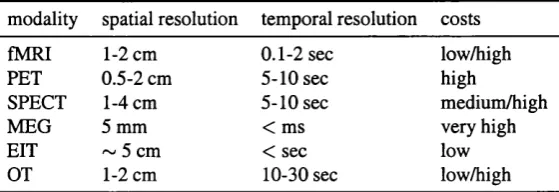
modality spatial resolution temporal resolution costs

fMRl 1-2 cm 0.1-2 sec low/high

PET 0.5-2 cm 5-10 sec high

SPECT 1-4 cm 5-10 sec medium/high

MEG 5 mm < ms very high

EIT ~ 5 cm < sec low

OT 1-2 cm 10-30 sec low/high

Ta b l e 1.1: Comparison o f different modalities for functional imaging (compiled from various sources).

1.4 Other Functional Imaging Techniques

Of course Optical Tomography is not the only modality for functional imaging. For comparison we shortly review other medical imaging techniques.

Structural versus functional imaging

In medical imaging we can make a distinction between,

• Structural imaging, where we are mainly interested in imaging anatomical structures. • Functional imaging, where we are mainly interested in imaging physiological changes in

the body.

Structural imaging modalities include x-ray imaging, magnetic resonance imaging and ultra­ sound that visualise for instance bone structure or different tissue types. Functional imaging modalities include for example PET, SPECT and Optical Tomography that for instance visualise the local glucose consumption or oxygenation state.

Overview of functional imaging modalities

Table 1.1 summarises current functional imaging modalities with their approximate spatial and temporal resolution. Currently, PET and fMRl are most popular for functional studies; in partic­ ular for brain studies. Below, we shortly describe the main modalities that are currently used for functional imaging.

C H A P T E R !. IN T R O D U C T IO N TO O P T IC A L T O M O G R A P H Y 37 the gamma photons, after which the data is used for tomographic imaging. The resolution is low, but SPECT has shown to be a useful clinical method to image regional changes in blood flow.

PET. Positron emission tomography is related to SPECT but here a compound is labeled with a positron emitting isotope. For example, labeled glucose, ^^F-fluorodeoxyglucose, is used to map out glucose metabolism and labeled water, H^^O, to map the blood flow. The positron quickly recombines with a nearby electron and during the annihilation process, two gamma rays are emitted, travelling in exactly opposite directions. The two gamma photons are simultaneously detected by a ring of ganuna-detectors, similar to PET, and used for tomographic imaging.

BOLD-fMRL The technique of blood oxygen level dependent{BOLD) imaging uses the prop­ erty that that the deoxyhaemoglobin molecule is slightly more paramagnetic than oxyhaemoglobin and thus give rise to small intensity changes in the MRI image. A problem is that these changes in contrast are generally very small; less than 15% at a magnetic field of 2 Tesla even when the haemoglobin oxygen saturation drops to 20% at acute hypoxia.

AST-JMRI. A different method using MRI that bears resemblance to tracer methods as in PET is known as arterial spin tagging (AST). However, in contrast to PET, no external tracer is needed but a preparatory radio-frequency pulse is applied which tags the protons in arterial blood that flows into the region of interest. AST selectively shows the increased flow in the capillaries, whereas BOLD primarily shows flow changes in the venules overlying the activated cortical area.

MEG. A magneto-encephalography (MEG) system typically consists of an array of super­ conducting quantum interference detector (SQUID) sensors. The SQUID sensors transcranially detect the tiny neuro-magnetic fields that arise from intracellular currents with a typical temporal resolution of milliseconds. The gravitational center of neuronal activity is determined by an in­ verse solution with accuracy of about 5 mm but the active region is mostly much larger. Currently, there are about 10-20 MEG systems in the US, and about 5-10 in Japan. The largest system to date has 512 magnetic sensors. The use of MEG is still only at experimental level, partly due to its very high costs.

C H A P T E R L IN T R O D U C T IO N TO O P TIC A L T O M O G R A P H Y 38 on very different physical phenomena, mathematically the imaging problem in EIT is very closely related with that in Optical Tomography. For some literature refer to, for example, Metherall et al [87].

1.5 Optical Tomography as a Nonlinear Ill-posed Inverse Problem

The general task of image reconstruction is to compute an image from the measured data. Imaging can be regarded as a parameter estimation problem or so called inverse problem.

The forward problem and inverse problem

A more rigorous treatment of the mathematics will be given in the next chapter. Here we shall be satisfied with a rather general treatment.

Suppose the data is described by a general vector y and that the image can be described by a general vector 0. Suppose that we also have a physical model that describes the relation between

0 and y , then we may write

y = V e (1.3)

where 7^ is a general operator that represents our physical model. Th& forward problem is then defined as to find the values of data y given image $.

In the image reconstruction problem, we are interested in the inverse problem. That is, to find the image 9, given the data y . Or we could write

e = V ~ ^ y (1.4)

where denotes the inverse or a pseudo-inverse operator.

In x-ray imaging 9 represents an absorption map of object, y will correspond to the measured attenuation projection, and the (linear) operator P is a so called Radon transform performing simple line integrals on the image (see for instance Barrett [18]). The inverse operator can be performed analytically using inverse Fourier transformation or using filter backprojection. See for example Brooks and DiChiro [29] for an introduction.

C H A P T E R L IN T R O D U C T IO N TO O P T IC A L T O M O G R A P H Y 39 intensities through, for example, the head when the optical properties of that head is given. How­ ever, the reconstruction problem is the inverse, we like to know what the optical parameters are

given the measured intensities around the interrogated the organ. The model operator V will be derived in the next chapter and we will see that it is based on the diffusion equation of heat transfer. An analytical form for the inverse operator does not exist in Optical Tomography because the problem is nonlinear.

Characterics of the OT inverse problem

To summarise, we may say that the inverse problem in Optical Tomography can be characterised by the following points:

• Ill-posedness. The diffusive nature of the photons is cause for the ill-posedness of problem. In practice this means that the obtained images have low resolution and are very sensitive to noise. ^

• Large-scale. The inverse problem typically deals with 1000 to several 10,000 parameters. • Non-linear. The inverse problem in Optical Tomography is highly nonlinear. This pre­

cludes the use of analytic methods such as back-projection methods.

• Dual-parameter. The optical property tissue is characterised by two parameters. Simulta­ neous reconstruction of both parameters complicates the inversion and may induce cross­ talk between the images.

Despite these mathematical and other practical difficulties, the promised advantages of a non- invasive oxygen monitor are huge and considerable efforts are still in progress.

1.6 Additional References

For a good introduction into the various aspects in Optical Tomography see for example a recent review by Yamada [138]. For a review more specific to measiu'ement techniques see Hebden et al [64] and for a review of mathematical modelling see for example Arridge et al [5]. For an ’An inverse problem is called ‘well-posed’ if it satisfies all Hadamard conditions [127]: (i) a solution exist, (ii) is

C H A P T E R !. IN T R O D U C T IO N TO O P T IC A L T O M O G R A P H Y 40 overview of aspects in the early developments in Optical Tomography see a collection of papers in [92].

The book edited by Webb [135] is a good general reference for medical imaging techniques. A paper by Brooks and DiChiro [29] provides a gentle and clear introduction to the mathematics of reconstruction techniques, but might be slightly outdated. For an overview of mathematical models for the different imaging modalities, see for instance Natterer [93]. More references on image reconstruction techniques will be given in Chapter 4.

Having a public, keeping a public in mind, means living in lies. (Milan Kundera)

C H A P T E R 2

P

h o t o n

M

i g r a t i o n

i n

T

i s s u e s

Our final objective is to be able to image the oxygenation state of interior tissue by interrogating an organ with near-infrared light. Before we can solve the imaging task, we need to understand

how light travels through tissue or more generally in a scattering medium. This chapter discusses the theory of light propagation in highly scattering media. We derive the mathematical formulas of the governing equations and introduce analytical and numerical methods for solving these.

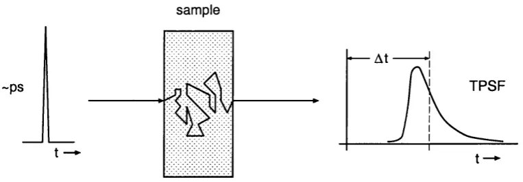
Figure 2.1 illustrates how a picosecond pulse is transmitted after propagation through a highly scattering medium. The pulse is generally delayed with delay time A i and the original pulse is now broadened. In Optical Tomography we call this time profile the temporal point spread function or TPSF.

sample

~ps

-— At

TPSF

t

Figure 2.1: Graphical representation of broadening o f a picosecond pulse propagating through a highly scattering medium.

C H A P TE R 2. P H O T O N M IG R A T IO N I N T IS S U E S 42

Chapter Outline

This chapter is a summary of general theory that will be needed in the subsequent chapters. Our goal in this chapter is to derive a partial differential equation (PDE) that describes the propagation of light in highly scattering media. All the presented material in this chapter is based on results from existing literature.

1. First, we need to determine which quantities parameterise the absorption and scattering properties of a medium. From electro-magnetic scattering theory we will derive the ab­ sorption coefficient, //&, and reduced scattering coefficient, //g.

2. Using iJ,a and jj.'g we formulate the transport equation (TE) that is the governing PDE for the distribution of photon density. Then we show that the diffusion equation (DE) is a sufficiently good approximation to the TE but much easier to calculate.

3. Then we introduce the hnite-elements method (FEM) as the preferred numerical method for solving the DE. We also derive an adjoint method for direct calculation of the gradient based on the FEM method.

2.1 Theory of Absorption and Scattering

This section reviews the general theory of electro-magnetic scattering and absorption. We dis­ cuss Mie and Rayleigh scattering and derive expressions for the absorption coefficient pa and scattering coefficient

ps-Physical origins of absorption

One of the material equations derived from Maxwell’s equation for electromagnetic theory states:

j = (jE , (2.1)

C H A P T E R 2. P H O TO N M IG R A T IO N I N T IS S U E S 43 while when cr ^ 0 the medium is said to be an electrical conductor. Metals have a very high value of (J so that light cannot cannot penetrate and gets mostly reflected.

Mathematically, a non-zero value of the specific conductivity will yield solution of the wave equation with exponentially decaying solutions with complex wave number k

where w is the angular frequency, c is the speed of light, p is the permeability and e is the permit­ tivity of the medium.

The absorption of light is due to interaction of electromagnetic waves with free electrons that are not bound to atoms. If energy is not dissipated, the electromagnetic waves will be re-emitted resulting in reflection of the light. In dissipating media, this energy is converted to heat.

Physical origins of scattering

By scattering we mean a change in the propagation distribution of incident light. At an atomic level scattering is closely related to absorption: a photon gets absorbed, but is almost instanta­ neously re-emitted. We do not consider inelastic scattering such as Raman scattering and fluores­ cence^ that change the frequency of the incident light.

Mie scattering theory

The previous paragraphs have explained the physical phenomena underlying absorption and scat­ tering at the atomic level. By using a complex wave number, k, we are able to fully characterise the propagation of waves in a medium. For instance, ignoring polarisation and assuming unit am­ plitude, a plane wave travelling in the z direction with given wave number k is simply described by,

E = exp{—ik z). (2.3)

C H A P TE R 2. P H O TO N M IG R A T IO N I N T IS S U E S 44 Rather than the plane wave solution, scattering theory is interested in how the field changes in presence of a scattering object. The analytical solution of the scattered field from a spherical object was obtained by Mie in 1908 and is referred to as the Mie theory. The derivation is quite straightforward but tedious; for a full account see, for example, Ishimaru [70]. We suffice by giv­ ing a general outline and greatly simplify the case by ignoring polarisation effects and considering only the two-dimensional case; the following is based of Bezuska [23].

Assume an incoming plane wave propagating in the z direction, as in Eq. 2.3, impinging on a spherical object with radius a. Now, we introduce a polar coordinate system centered at the sphere with spherical coordinates (r, 6) and write the expansion of the plane wave using Bessel^ functions, J„, which form the radial basis functions and Legendre polynomials^, P„(cos0) = cos nO, which form the angular basis functions

Ei = exp ik z

oo

= ^ 2 i^Jn{kr) cos nO (2.4)

n = 0

This expansion uniquely defines the plane wave. Now, we introduce a scattered wave inside, Er,

and a wave. Eg, outside the sphere both also in polar coordinates using a similar expansion,

oo

Er = ^ 2 CLnJn i^'r) COS nO

n = 0 oo

Eg = ^ 2 ^ n IIn { k r ) cos nO (2.5)

n = 0

where are Hankel functions of the first kind, k' is the wave number inside the sphere and and bn are coefficients yet to be determined.

The unknown coefficients and bn can be determined by imposing boundary conditions'^ that require continuity of electric vector E and magnetic vector H across the boundary r = a.

After determination of On and bn the scattered wave is completely described. While the ^Bessel functions are special functions that form an orthonormal basis for the radial coordinate in a polar coordinate system. It is helpful to think of Bessel and Hankel functions as cousins of “sine” and “cosine” but for the radial coordinate in 2D. In 3D, the Bessel functions generalise to spherical Bessel functions.

^Legendre polynomials, Pn{x), form an orthogonal basis for —1 < x < 1. It is helpful to think them as “cousins” of the power terms x^. The first few Legendre polynomials are: Po(x) = 1, P i(x) = x, and P2{x) = |(3x^ — 1). But simplify for x = cos 6 to: Pn (cos 9) = cos n9.