Strain gradient elasticity with geometric nonlinearities and its computational evaluation

(1)

R E S E A R C H A R T I C L E

Open Access

Strain gradient elasticity with geometric

nonlinearities and its computational

evaluation

B Emek Abali

1*

, Wolfgang H Müller

1

and Victor A Eremeyev

2

Abstract

Background: The theory of linear elasticity is insufficient at small length scales, e.g., when dealing with micro-devices. In particular, it cannot predict the “size effect” observed at the micro- and nanometer scales. In order to design at such small scales an improvement of the theory of elasticity is necessary, which is referred to asstrain gradient elasticity. Methods: There are various approaches in literature, especially for small deformations. In order to includegeometric nonlinearitieswe start by discussing the necessary balance equations. Then we present a generic approach for obtaining adequate constitutive equations. By combining balance equations and constitutive relations nonlinear field equations result. We apply a variational formulation to the nonlinear field equations in order to find aweakform, which can be solved numerically by using open-source codes.

Results: By using balances of linear and angular momentum we obtain the so-called stress and couple stress as tensors of rank two and three, respectively. Since dealing with tensors an adequate representation theorem can be applied. We propose for an isotropic material a stress with two and a couple stress with three material parameters. For understanding their impact during deformation the numerical solution procedure is performed. By successfully simulating the size effect known from experiments, we verify the proposed theory and its numerical implementation. Conclusion: Based on representation theorems a self consistent strain gradient theory is presented, discussed, and implemented into acomputational reality.

Keywords: Size effect, Micromechanics, Constitutive equations

Background

Traditional constitutive models relating stresses and strains are independent of the size and shape of the con-tinuous body. For example, we model the linear response at small deformations with HOOKE’s law, which has the same form for huge and small structures. Unfortu-nately, such a simple approach becomes inadequate at the micrometer scale. One of the basic approaches in statics, the so-called EULER-BERNOULLIbeam theory, results in inaccurate solutions at very small dimensions. For exam-ple, sub-micrometer structures frequently show a stiffer response than predicted by traditional theory. This so-calledsize effecthas been known experimentally for a long

*Correspondence: [email protected]

1Technische Universität Berlin, Institute of Mechanics, Einsteinufer 5, D10587 Berlin, Germany

Full list of author information is available at the end of the article

time, see, e.g., (Morrison et al. 1939). Formally, the size effect can be modeled by material properties that depend on specimen size. However, in order to include the size effect in a more rational manner, we will generalize the theory of elasticity by means of higher gradient terms. In fact, theories of higher gradients were proposed more than four decades before, cf., (Mindlin and Tiersten 1962; Mindlin and Eshel 1968). They are still under discussion. Moreover, various variants were developed over the last decades, see for an overview (Gurtin et al. (2010), §90). Especially in micromechanics an applicable theory of gen-eralized theory of elasticity becomes necessary, as pointed out by (McFarland and Colton 2005).

We shall discuss deformation and its description in terms of higher gradients of displacement within the framework of continuum mechanics principles. First, we present the balance equations of linear momentum and

(2)

angular momentum, and identify their flux terms as stress and couple stress, respectively. Second, when deriving constitutive equations for the stress and the couple stress we use tensorial relations. Balance equations in combi-nation with constitutive equations will result in nonlin-ear field equations. Third, in order to solve these field equations we generate aweakform by using a variational formulation. For the weak form discretization in time is performed by making use of thefinite difference method. For discretization in space the finite element method is used. Fourth, we implement a code in Python, see (Jones et al. 2001), by using a novel collection of open-source packages distributed under the FEniCS project, see (Logg et al. 2011). We publish the code in (Abali 2015) under GNU Public license as stated in (Gnu Public 2007) in order to encourage further studies.

Methods

Governing equations

We apply the standard nomenclature of continuum mechanics including the summation convention on repeated indices and use the initial positions of particles, X, as reference frame where all functions are evaluated. Consider a continuum body deforming from itsknown ini-tial frame,B0, to anunknowncurrent frame, B, in time,

t. All particles move from their initial positions,X, to the current positions,x = x(X,t). We apply Cartesian coor-dinates and choose two particles 1 and 2 with current positions:

1

xi=xi(

1

Xj,t),

2

xi=xi(

2

Xj,t), i,j=1, 2, 3 . (1)

The distance between these particles reads

x=xixi, xi=

1

xi−

2

xi . (2)

The current distance vector, xi, can be expressed by

expanding the position of one particle about the position of the other particle by using a TAYLORseries:

1 xi=xi

₁ X,t

=xi

₂ X,t

+∂2xi

∂Xj

2

X,t

₁ Xj−

2 Xj

+ +1₂ ∂2xi

∂Xj∂Xk

2

X,t

₁ Xj−

2 Xj

1 Xk−

2 Xk

+O

(X1 −X2 3

,

1 xi−

2

xi=xi= ∂

xi

∂Xj

Xj+

1 2

∂2_x

i

∂Xj∂Xk

XjXk+O(X3),

(3)

withXi =

1

Xi −

2

Xi. If the initial and current distances

become infinitesimal,Xi →dXiandxi→dxi,

respec-tively, we obtain the transformation property for the line element by neglecting second order terms:

dxi=Fij dXj, Fij= ∂ xi ∂Xj

, (4)

where the deformation gradient,Fij, has been introduced

as transformation between the line elements (distances) in the initial and current frames. This transformation leads to the transformation of the current surface element, dai,

and volume element, dv, onto the initial surface element, dAi, and volume element, dV, such that:

dai=(F−1)kiJdAk, dv=JdV, J=det(F). (5)

In local continuum mechanics it is assumed that the

particles interact within the local neighborhood, where the distance becomes infinitesimal such that the first gradient describes the behavior of material accurately. We can generalize the behavior by including the sec-ond gradient, which enables an interaction of particles in a greater neighborhood. This theory is nonlocal and we need different equations restricting the first and the second gradients.

The formulation is easier to develop in displacements,

ui =xi−Xi, we introduce

ui,j= ∂ xi ∂Xj −δij

, ui,jk= ∂

2_x

i ∂Xj∂Xk

. (6)

The quantities ui,j and ui,jk are independent locally,

because we cannot determine the derivative of a func-tion at a point just by knowing its value at that point. Since these two quantities are independent, we need two governing equations. We propose to apply two balance equations of momenta in the current frame:

Bp

lin.

i dv •

=

∂Bσjidaj+

Bρfidv, (7)

Bp

ang.

i dv

•

=

∂Bαjidaj+

Bρzidv,

where plin._i ,σij, fi are the linear momentum density (per

volume), the flux of linear momentum, and the supply of linear momentum, respectively. pang._i , αij, zi denote

the angular momentum density, the flux of angular momentum, and the supply term of angular momentum, respectively. The linear momentum density,plin._i , and the angular momentum density, pang._i , are conserved quan-tities, i.e., they are given in balance equations without production terms. They can be rewritten by using the spe-cific (per mass) linear momentum and the spespe-cific angular momentum:

plin._i =ρvi, pang._i =ρai. (8)

Moreover, the specific angular momentum is decom-posed into an intrinsic specific spin, si, and into the

moment of (specific linear) momentum:

ai =si+ijkxjvk, (9)

where we have introduced the LEVI-CIVITAsymbol,ijk.

(3)

tensor. Following (Müller (1973), Ch. II,§2.d) we can mul-tiply the balance of linear momentum in its local form by

ijkxjand subtract the result from the balance of angular

momentum for acquiring a balance of spin. The produc-tion term of the spin readsijkσjk. For non-polar media the

spin and its production vanish, i.e.,si=0 andijkσjk =0.

This assumption leads to a symmetric CAUCHYstress ten-sor,σij = σji. A non-polar medium has no intrinsic spin

such that the continuum possesses three degrees of free-dom given by the displacement,ui. For structures on the

macroscale the balance of linear momentum is sufficient for calculating the displacement. The balance of angu-lar momentum is automatically satisfied by a symmetric CAUCHYstress tensor, in other words, the flux of angu-lar momentum is assumed to vanish. For structures on the microscale this assumption must be rediscussed and a model for the flux of angular momentum needs to be implemented.

The balance Eqs. 7 can be transformed onto the refer-ence frame by using the solution for the balance of mass,

ρ0 = ρJ, with J = det(Fij). After applying GAUSS’s

theorem we obtain in every regular point ofB0:

ρ0∂

vk

∂t −

∂Prk ∂Xr −ρ0

fk=0 , Prk =(F−1)rjJσjk, (10)

ρ0∂

ak

∂t −

∂Ark ∂Xr −ρ0

zk=0 , Ark =(F−1)rjJαjk.

Since the angular momentum consists of the spin and the moment of (linear) momentum, the flux of angular momentum,Aij, can be decomposed into two parts where

the first part is a flux of spin,μij, and the second part is

the moment of the flux of (linear) momentum:

Ark =μrk+kjiXjPri. (11)

The flux of spin,μij, is usually called a couple stress, as

in (Mindlin and Tiersten 1962). Analogously, the supply of angular momentum reads

zk=lk+kjiXjfi. (12)

By following CAUCHY’s tetrahedron argument, as in (Truesdell and Toupin (1960), Sect. 203), we relate the stress to a traction on the surface,ti, and, analogously, the

couple stress to a moment couple on the surface,mi:

σij=nitj, μij=nimj. (13)

Note that the moment couple mj is an axial vector

(pseudovector). Thus, it does not have the same trans-formation properties as a polar vector (tensor of rank one). Therefore, instead of the axial vectors,ai, mi, we

use, as in (Truesdell and Toupin (1960), Sect. 203), the skew-symmetric form that is well-known in rigid body dynamics for the representation of the angular velocity.

We change the balance of angular momentum in the reference frame into the skew-symmetric form:

ρ0∂

aik

∂t −

∂Airk ∂Xr −ρ0

zik =0 , (14)

with:

aik =

1

2ikjaj, Airk= 1

2ikjArj, zik = 1

2ikjzj. (15) Now by using the tensor identity:

ikjjmn=jikjmn=δimδkn−δinδkm, (16)

we obtain

Airk=

1 2ikjμrj+

1

2ikjjmnXmPrn=μirk

+1

2(XiPrk−XkPri)=μirk+X[iPrk], zik=

1 2ikjlj+

1

2ikjjlmXlfm=lik+ 1

2(Xifk−Xkfi)=lik+X[ifk]. (17)

Since we deal with a non-polar medium the specific angular momentum simplifies to

aik =

1 2ikjaj=

1

2ikjjlmXlvm= 1

2(Xivk−Xkvi)=X[ivk]. (18)

The skew-symmetric form was presented in a similar way in (Mindlin and Eshel 1968; Toupin 1962), (Truesdell and Toupin (1960), Sect. 205). However, the starting point and the motivation are different here.

The objective is to find such a displacement field,ui = xi−Xi, so that Eq. (10)1and Eq. (14) are satisfied. By using the time rate of displacements as the velocity:

vi= ˙xi= ˙ui, sinceX˙i=0 , (19)

and by employing a comma for denoting the partial derivatives inXithe balance equations of momenta read

ρ0¨uk−Prk,r−ρ0fk=0 ,

ρ0X[iu¨k]−μirk,r−P[ik]−X[iPrk],r−ρ0lik−X[ifk]=0 . (20)

Since we will solve both of them simultaneously we can subtract the first one multiplied byX[i from the second

one and obtain

ρ0u¨k−Prk,r−ρ0fk=0 , −μirk,r−P[ik]−ρ0lik =0 . (21)

These equations of motion include supply terms,fi,lij, to

be given and flux terms,Pij,μijk, to be defined with respect

to the displacement (or its gradient). Only then Eqs. (21) are closed and can be solved.

Constitutive relations

(4)

μijk. The main objective of the whole theory is to find

the displacement,ui. Therefore, the constitutive equations

shall depend onui,jandui,jk—this dependence is

consis-tent with the motivation of the theory leading to Eqs. (6). Instead of ui,j we can employ the GREEN-LAGRANGE

strain:

Eij=

1

2(Cij−δij), Cij=FkiFkj, (22)

which is obviously symmetric. Instead ofui,jkwe can apply

the gradient of the GREEN-LAGRANGEstrain,Eij,k. Hence,

the stress tensor and the couple stress tensor may depend on the strain and its gradient. We want to find out their general form forlinearandisotropicmaterials. For a lin-ear isotropic material the dependence of the stress on the strain gradient vanishes, as well as the couple stress fails to depend on the strain, see (dell’Isola et al. (2009), Sect. 3). Since the strain is a symmetric tensor,Eij=Eji, we use the

second PIOL A-KIRCHHOFFstress tensor,Skj=(F−1)jiPki,

which is also symmetric, Sij = Sji, based on the

defini-tion of the first PIOL A-KIRCHHOFF stress tensor,Pij, in

Eq. (10)2. Hence the general linear relations for the stress and the couple stress read

Sij=CijklEkl, μijk =DijklmnElm,n. (23)

By following (Suiker and Chang 2000) we acquire the general tensorial form of isotropic tensors of rank four and six, i.e., forCijkl andDijklmn, respectively. For the sake of

brevity we skip the detailed explanation that can be found in the Appendix starting on p. 9. An isotropic tensor of rank four from Eq. (68) on p. 10 reads

Aijkl=c1δijδkl+c2δikδjl+c3δilδjk. (24)

We can use this form forCijkland obtain the constitutive

equation betweenSijandEijin Cartesian coordinates:

Sij=CijklEkl, Cijkl=λδijδkl+μδikδjl+νδilδjk. (25)

Since Eij = Eji we conclude that μ = ν and obtain

ST. VENAN T’s law for elasticity:

Sij=λEkkδij+2μEij, (26)

where the LAMÉ parameters, λ, μ, are determined by using engineering constants, namely YOUNG’s modulus,

E, and POISSON’s ratio,ν:

λ= ₍ Eν

1+ν)(1−2ν) , μ=

E

2(1+ν). (27)

Next we findDijklmnfor isotropic materials by using the

same procedure. We apply the relation in Eq. (70) on p. 15 forD_ijklmnin Eq. (23)2, and obtain

μijk=c01δijEkm,m+c02δijElk,l+c03δijEll,k+c04δikEjm,m+

+c05δikElj,l+c06δikEll,j+c07δjkEim,m+c08Eij,k+

+c09Eik,j+c10δjkEli,l+c11Eji,k+c12Eki,j+

+c13δjkEll,i+c14Ejk,i+c15Ekj,i.

(28)

Fifteen parameters, c01. . .c15, need to be determined. SinceE_lm_,_n=E_ml_,_nwe obtain

μijk =(c01+c02)δijEkm,m+c03δijEll,k+(c04+c05)δikEjm,m+

+c06δikEll,j+(c07+c10)δjkEim,m+(c08+c11)Eij,k+

+(c09+c12)Eik,j+c13δjkEll,i+(c14+c15)Ejk,i.

(29)

Hence the most general form of the couple stress or the flux of spin for linear elasticity has nine phenomeno-logical constants. Quite often two more assumptions are made. First, one takes μijk ≈ μjik for granted. Second,

one assumes that μijkEij,k is a part of the

(deforma-tion) energy, such that Dijklmn = Dlmnijk holds. Under

these assumptions nine constants reduce to five material constants, see (dell’Isola et al. (2009), Eqs. (3.1)–(3.7)) and for an overview of such theories refer to (Askes and Aifantis (2011), Sect. 2). We try to avoid introducing assumptions restraining the formulation to specific type of materials.

In the last section we have obtained the governing equations. There have been some assumptions, which bring in further restrictions in order to make the form of Dijklmn admissible with Eqs. (21). We can neglect the

supply term l_ik or at least restrict it to be antisymmet-ric,l_ik = −l_ki. Hence we observe by inspecting Eq. (21)2 thatμijk has to be antisymmetric in the indicesi,k, i.e., μijk = −μkjior equivalentlyμijk+μkji=0. This condition

implies

c01+c02= −(c07+c10), c03= −c13,

c04+c05=c06=c09+c12=0, c08+c11= −(c14+c15). (30)

After employing these restrictions and renaming the constants the couple stress reads

μijk =α δijEkm,m−δjkEim,m

+β δijEmm,k−δjkEmm,i

+ +γ Eij,k−Ejk,i

.

(31)

In a heterogeneous material the material parameters,α,

(5)

and investigate their roles in deformation. The constitu-tive Eq. (31) for the couple stress tensor and Eq. (26) for the stress tensor will be implemented in the numerical investigation.

There is a well-known material equation for the cou-ple stress with one parameter, see for examcou-ple (Gao and Park 2007):

μijk =cSjk,i, (32)

which is actually a special choice of the parameters of Eq. (31),α,β, andγ. In order to see this we insert Eq. (31) and Eq. (26) into Eq. (32) as follows

α δijEkm,m−δjkEim,m

+β δijEmm,k−δjkEmm,i

+ +γ Eij,k−Ejk,i

=cλEll,iδjk+2cμEjk,i.

(33)

One possible choice ofα,β,γ can be obtained by multi-plying Eq. (33) withδijand by using a direct analysis with

the assumption ofα=βsuch that:

2αEkm,m+2βEmm,k+γEii,k−γEik,i=cλEmm,k+2cμEik,i,

2α−γ =2cμ, 2β+γ =cλ, if :α=β ⇒ α=β=c

_λ

4+

μ

2

, γ =c _λ

2−μ

.

(34)

Another possible choice results analogously by multi-plying Eq. (33) withδjkand, again, by assumingα = βas

follows

−2αEim,m−2βEmm,i+γEik,k−γEkk,i=3cλEll,i+2cμEkk,i,

−2α+λ=0 , −2β−λ=3cλ+2cμ, if :α=β ⇒ α=β= −c

3 4λ+

μ

2

, γ=−c

3 2λ+μ

.

(35)

Therefore, the constitutive Eq. (32) is a special choice of the proposed relation in Eq. (31). Of course the assump-tionα=βis difficult to justify. Thus we will use the more general formulation given by Eq. (31).

In the following section we will implement the balance Eqs. (21) complemented by the constitutive equations:

Sij=λEkkδij+2μEij,μijk=α δijEkm,m−δjkEim,m+

+β δijEmm,k−δjkEmm,i+γ Eij,k−Ejk,i

(36)

in a numerical computational environment that allows us to comprehend the role of the parametersα,β,γ.

Computational approach

There are various numerical implementations of theories dealing with higher order materials. We skip a discussion of pros and cons between different implementations and refer to (Askes and Aifantis (2011), Sect. 5) instead. In this

work we solve the balance equations complemented by the constitutive equations numerically in a discrete fashion, viz., by using the finite element method in space and the finite difference method in time. First, we obtain the so-calledweakform for Eqs. (21) within a finite domain,, in a standard manner by multiplying them with correspond-ing test functions and by performcorrespond-ing integration by parts on the flux terms:

F1=

ρ0u¨kδuk+Prkδuk,r−ρ0fkδuk

dV−

∂PrkδukNrdA,

F2=

μirkδuk,ir−P[ik]δuk,i−ρ0likδuk,iδuk,i

dv−

∂μirkδuk,iNrdA.

(37)

The choice of the test functions can also be based on introducing a new field such as a rotation instead ofδuk,i,

see for example (Bauer et al. 2012). However, because we want to determine the displacement field there is no reason or computational benefit to introduce another quantity such as a rotation field. Therefore, we useδuk,i

and obtain two integrands in Eqs. (37) in the same unit of energy density. Hence we can sum them up:

F=F1+F2. (38)

The weak form, F, is of second-order in space regarding the displacement field. Therefore, we choose finite ele-ments of the continuous GALERKINtype of second poly-nomial degree. In other words, the displacements and also their test functions are from a HILBERTspace,ui,δui ∈ H2_{as described in (Hilbert 1902). Moreover, their} gradi-ents have to exist, i.e., more specifically the solution space is a SOBOLEV space within the finite domain, referred to as finite elements. Elements are discrete subdomains,

i _∩j _{= {}}_, _∀_i ₌ _j_{, which collectively constitute the}

region,e=B0, where the computation takes place. For the time discretization we use thefinite difference

method:

∂(·)

∂t =

(·)−(·)0

t , t=t

(k+1)₋_t(k)_, ₍₃₉₎

where time is discretized as a list of length n equally separated,t(k)= {t, 2t,. . .nt}. This approach is sim-ple and stable for real-valued problems because it is an

implicitmethod. In order to see this, we can apply a TAY

-LORexpansion to the value (in any position) at the time instantt(k)in order to find the value (in the same position) at the time instantt(k+1)as follows

ui

xi,t(k)

=ui

xi,t(k)+t−t

=ui

xi,t(k+1)−t

= =ui

xi,t(k+1)

−t∂ui ∂t

xi,t(k+1)

,

(40)

(6)

is sought, it is an implicit method. Obviously by rewriting the latter we acquire Eq. (39) for the time discretization. We employ the GALERKINtypefinite elementmethod, so that the test functions are chosen from the same SOBOLEV space as the displacements. Hence, the notation,δui, gets

a fully consistent meaning. The weak form discretized in time and space by integrating over each finite element,e, and assembling by summing them up reads

F=

elements

e

ρ0ui−2u 0 i+u00i

tt δui+Pjiδui,j−ρ0fiδui+μijkδuk,ij−

−P[ik]δuk,i−ρ0likδuk,i

dV−

∂ Pjkδuk+μijkδuk,i

NjdA.

(41)

Since the latter functional or weak form is nonlinear in

ui we can only solve it by using a linearization. We use a

NEW TON-RAPHSONlinearization scheme at the level of differential equations. In other words, this linearization is implemented before the assembly operation (build-ing matrices). Therefore, the success of the linearization depends only on the starting value for approximation. Since we solve the problem transiently the starting value is either the initial condition, which is exact, or the solu-tion from the last time step, which is exact up to machine precision. The NEW TON-RAPHSON linearization can be realized as an expansion of the functional, F= F(ui,δuj),

for finding the values in the next time step,ui(t+t). For

a sufficiently smalltthis can be rewritten into:

ui(t+t)=ui(t)+ui(t). (42)

If the change,ui, is small then the above relation yields

the correctui(t+t). If this is not the case, then we can

solve it incrementally until|ui| is smaller than a given

value (tolerance). For a small time step,t, this incremen-tal approach leads to the correct solution. In order to find the increment,ui, we can again employ a TAYLORseries

truncated after linear terms on the functional:

F(ui+ui,δui)=F(ui,δui)+Jiui, (43)

where the JACOBIan,Ji, is simply the derivative of F with

respect to the unknowns,ui. Since the weak form shall be

zero:

F(ui,δui)+Jiui=0 , (44)

we have obtained an equation linear in the increment,

ui, which is solvable. By updating the solution:

ui:=ui+ui, (45)

and solving the increment once more until the value is smaller than the given tolerance, we determine the cor-rect value ofui(t+t). We have programmed in Python

and computed by using the novel collection of open-source packages, developed under FEniCS project (Logg

et al. 2011). Thedirectionalderivative,Jiui, is calculated

by using the following procedure:

Jiui=

d

daF(ui+aui,δui)

a=0

. (46)

This approach is fully automatized by using a symbolic derivation, see (Alnaes and Mardal 2010). Therefore, the only necessary input is the weak form given in Eq. (41). All 3D-visualizations are realized by using ParaView.1 All 2D-plots were created by MatpPlotLib packages, see (Hunter 2007), developed for NumPy, see (Oliphant 2007). The code used for solving the examples in the next section is published in (Abali 2015) under GNU public license as declared in (Gnu Public 2007).

Results

In order to analyze the effect of the material parameters,

α,β,γ in the proposed constitutive equation for the cou-ple stress μijk we construct a simple example to solve.

Consider a three-dimensional beam clamped on one end which deforms when subjecting it to a shear loading on the other end. The beam is of length 10μm. It is a slen-der beam since its width/length and height/length ratios are both 1/30. For all calculations we use the material parameters of generic aluminum:

ρ=2700·10−15g/μm3, E=72 GPaˆ=mN/μm2, ν=0.33 . (47)

We analyze three different loadings, viz., shear loading, tensile loading, and torsion. The loading has been imple-mented as a NEUMANNboundary condition at the end of the beam in Eq. (41) by defining a traction vector, ˆti, as

follows ˆ

t_k =P_jkNj (48)

Since the other boundaries are free the traction vanishes. Analogously a traction for the couple stress can be defined

ˆ

τki=μijkNj (49)

causing a spin on the boundaries by applying a moment at the micron scale. For free boundaries as well as for the both ends we assume that the system is lacking such a traction. We employ homogeneous NEUMANN, in other words,naturalboundary conditions for the couple stress term. For each one of the loadings we have performed four simulations:

Sim. I (color: gray) :_α₌0 mN , _β₌0 mN , _γ ₌0 mN , Sim. II (color: red) :α= −1 mN , β=0 mN , γ =0 mN , Sim. III (color: green) :α=0 mN , β= −1 mN , γ =0 mN , Sim. IV (color: blue) :α=0 mN , β=0 mN , γ = −1 mN .

(7)

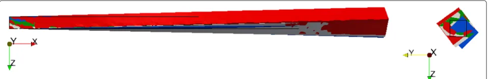
Fig. 1Shear loading. The initial shape of the beam is outlined by black lines. Gray (Sim. I), red (Sim. II), green (Sim. III), blue (Sim. IV) beams present the 50 times upscaled deformed shape with different material parameters

For each loading case we present all simulations and by comparing them we try to comprehend the effects of theα,β,γ parameters on the deformation. We start with shear loading. The beam lies along thex-axis and the load-ing at the tip is applied inz-direction. All simulations can be seen in Fig. 1.

The initial shape is denoted by black lines. The classical beam bending (without couple stress) is colored in gray for comparison. The parameterα= −1 (red) has an insignif-icant effect relative to the parametersβ= −1 (green) and

γ = −1 (blue). The green and blue colored deformations present an additional bending, such that the amount of bending onyz-plane decreases. In other words, the beam responds stiffer to shear loading in case of existingβorγ parameters.

Next we analyze tensile loading. The same configura-tion for simulaconfigura-tions has been used and the results are presented in Fig. 2 by using the same colors.

The initial geometry is again denoted by black lines, we have tilted the geometry for better visualization. The gray deformation is the classical stretching without couple

stress. The effect ofα(red) is significant again by causing an additional bending motion. Relative to the effect ofα the effects ofβandγ can be neglected.

Finally we analyze torsion. Four simulations with the previous color codings are depicted in Fig. 3.

The initial shape can be seen in black lines in the front view. In this case γ (blue) causes the most significant deviation from the classical solution (gray) without couple stress.

By observing the three loading cases we can conceive possibilities for measuring the parameters,α,β,γ. During shear loading the effects due to theαandγparameters are smaller than the effect ofβ, such that it may be neglected. For tensile loading the effects ofβandγ are smaller than

α and may be ignored. In torsion the effect of α is sig-nificant and the effects of β and γ may be neglected. Under these simplifications the parameterα (red) can be measured by a tensile test by assuming that green and blue deformations are the same as the gray deformation in Fig. 2. The parameterβ (green) can be measured by a shear test with the simplification that the red, blue, and

(8)

Fig. 3Torsional loading. The initial shape of the beam is outlined by black lines. Gray (Sim. I), red (Sim. II), green (Sim. III), blue (Sim. IV) beams present the 50 times upscaled deformed shape with different material parameters

gray deformations are the same in Fig. 1. The parameter

γ (blue) could be measured by a torsion test under the assumption that the red and green deformations in Fig. 3 are the same as the gray deformation.

The proposed strain gradient theory is an extension of the classical elasticity theory. Therefore, in the limit, strain gradient theory has to correspond to the classical theory of elasticity. In other words, the effect of couple stress should decrease while increasing the size of the geometry. We can examine the correspondence between strain gradient and classical elasticity by using an analytic solution. The EULER-BERNOULLI beam theory presents a closed-form solution for a slender beam in elastostat-ics. If the geometry is such that the length, , is ten times more than its width and thickness, then the beam can be considered as being slender. The deflection, w, of such a beam is well known as a function along the axis:

w= F

3 6EI

3x

2 −x3

, (51)

where the load, F, is the bending force shearing at tip of the beam, x = , and the modulus of elas-ticity E together with the moment of inertia I result in a bending rigidity EI along the axis of the deflec-tion. We consider a rectangular cross sectional area with width and height, b, h, respectively. The bending is on the axis along the width so that the moment of inertia becomes

I= bh

3

12 . (52)

By inserting the moment of inertia, we obtain

E= 4F

bumax.

z

h

3

, (53)

if we consider the deflection at the end of the beam,w(x= ) = umax._z . Since the modulus of elasticity shall be con-stant in classical beam theory we can compute umax._z by an appropriate simulation for a three-dimensional contin-uum body with varying beam’s length(and holding the geometric ratio fixed, /h = 30). According to classical beam theory the ratio of shearing force to deflection at

the tip shall be constant in beam’s length. However, exper-imental results demonstrate that a smaller beam presents a stiffer behavior, see (Lam et al. 2003) and McFarland and Colton (2005). We have observed thisstiffening phe-nomenon in Fig. 1 for one specific length. Now we vary the length for the beam and examine the correspondence of strain gradient theory to classical elasticity by using the following parameters:

ρ=2700·10−15g/μm3, E=72 GPaˆ=mN/μm2, ν=0.33 ,

α=0 mN , β= −1 mN , γ =0 mN .

(54)

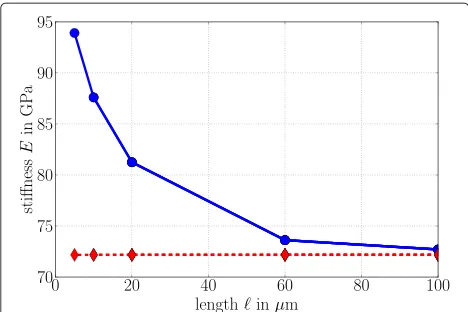
The numerical results have been compiled in Table 1. Due to the parameter β the size effect is significant and it is qualitatively consistent with the experimental results presented in (Lam et al. (2003), Fig. 12). In Fig. 4 we demonstrate this by simulating withβ= −1 mN (with couple stress) and also withβ = 0 mN (without couple stress) in order to verify that the code works as expected.

As discussed previously the stiffening behavior is due to additional bending resulting from the couple stress. How-ever, this bending does not affect the curvature. We have observed this behavior by plotting the normalized (with respect to the tip deflection)z-displacement of each beam. Since the curvature remains the same, we omit to present the results.

We emphasize that the material constant,E, does not change in reality. This example demonstrates that the beam when treated as a continuous body by using strain gradient elasticity responds stiffer than predicted by the EULER-BERNOULLIbeam theory.

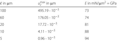
Table 1Variation of YOUNG’s modulus predicted by the EULER-BERNOULLIbeam theory for the ratio/h=/b=30 in case of changing the length of the beam

inμm umax

z inμm Ein mN/μm2= GPa

100 495.19·10−3 73

60 176.05·10−3 74

20 17.72·10−3 81

10 4.11·10−3 88

(9)

Fig. 4Stiffening due to the size effect. The blue dots (connected with the continuous line) denote simulations withβ= −1 mN and the red diamonds (connected with the dashed line) are computed by setting β=0 mN. By increasing the length of beam,, the strain gradient corresponds with the classical theory

Conclusion

We have briefly outlined strain gradient elasticity from a continuum mechanics perspective. Starting from the balances of momenta we have obtained the so-called stress and couple stress tensors (of rank two and three, respectively). By applying general tensor relations we have obtained the necessary constitutive equations for the stress and for the couple stress. It is significant that we have proposed a couple stress with three material parame-ters, viz.,α,β, andγ. In order to comprehend their impact during deformation we have implemented a numerical solution procedure where the discretization in time has been combined with the finite difference method. The dis-cretization in space was realized with the finite element method. By simulating different loading cases we analyzed the couple stress parameters. We also verified the pro-posed theory qualitatively by establishing a simulation of the size effect.

There have been three main difficulties that we have overcome with some assumptions and left their discus-sions to further studies. The first difficulty arises by moti-vating a flux of spin in a non-polar medium. Since spin fails to exist in a non-polar medium and since we have assumed that the CAUCHYstress tensor is symmetric (so that the spin production vanishes), it is rather difficult to justify why the flux of angular momentum (couple stress) should exist. Nonetheless, our objective has been the modeling of couple stress for a non-polar medium. The second difficulty lies in determining a description for a measurement procedure for the material parame-ters in the proposed couple stress, namely α, β, γ. We have discussed their possible measurement after some assumptions, whereαis determined by tensile,βby shear,

andγ by torsion. However, the correctness of simplifi-cations based on these assumptions is difficult to test. The third difficulty arises by varying the material param-eters in order to comprehend their roles quantitatively. Their effects seem to be counter-intuitive and difficult to explain in a straightforward way. Numerical problems arise by choosing positive or greater values for the param-eters. Unfortunately, we could not find general conditions in order to restrict the possible values of parameters. For using positive definiteness or thermodynamical laws we need to define the energy due to the spin. Spin is assumed to vanish and the stored energy is not uniquely defined for strain gradient theory. Therefore, the verification of the chosen parameters, and thus, the validation of presented results seem to be more difficult than expected. Any quan-titative verifications by using experiments have been left to further research.

Endnote

1_{http://www.paraview.org}

Appendix

A EUCLIDian transformation expressed in a Cartesian coordinate system:

xi =Oijxj+bi , Oij=Oij(t), bi =bi(t), ∂

xi

∂xj =

Oij,

(55)

results in anobjectivetensor being transformed as:

Aijk...r =OiiOjjOkk. . .OrrAijk...r, (56)

whereOijis a rotation tensor,O−1=OTand det(O)=1,

between two Cartesian coordinate systems characterized

by orthonormal base vectors. An arbitrary tensor, B, is

referred to as anisotropictensor if its components in any

orthogonalcoordinate system transform such that:

Bijk...r =QiiQjjQkk. . .QrrBijk...r, (57) B_ijk_..._r=B_i_j_k_..._rQ_i_iQ_j_jQ_k_k. . .Q_r_r,

whereQij is a proper transformation between two

arbi-traryorthogonalcoordinate systems. Therefore, an objec-tive tensor is isotropic under rotations:

Aijk...r =OiiOjjOkk. . .OrrAijk...r, (58) Aijk...r=Aijk...rOiiOjjOkk. . .Qrr.

Every even or oddformal orthogonal invariant polyno-mialfunction depending onnvectors:

F=Fa(_i1),a_i(2),. . .,a(_in) , (59)

can be represented in a linear form:

(10)

where the scalar functions, F1, F2, . . . , Fm, are built

by two different combinations of its arguments,

a(_i1),a_i(2),. . .,a(_in). The first combination is the sum of scalar products of every set of two vectors:

a(α)·a(β)=δija(α)i a (β)

j , α=β. (61)

The second combination is to use the determinant for every set oflodd vectors:

deta(_i1)a_j(2). . .a(_rl)=ij...ra(i1)aj(2). . .a(rl). (62)

In the Cartesian coordinate system the KRONECKER symbol,δij, is the metric tensor:

δij=

1 if i=j

0 otherwise , (63)

and the LEVI-CIVITAsymbol,ij...r, is equal to the

permu-tation symbol:

ij...r=

⎧ ⎨ ⎩

+1 if ij. . .ris an even permutation of 1, 2,. . .m

−1 if ij. . .ris an odd permutation of 1, 2,. . .m 0 otherwise

.

(64)

Both,δijandij...r, are isotropic tensors, therefore, the

following relation holds for an isotropic tensor,Aij...r:

Fa(1),a(2),. . .,a(n)

=Aij...ra(i1)aj(2). . .a(rn). (65)

Consider an isotropic tensor of rank two,Aij. We apply

the procedure:

Aija(_i1)a(_j2) = F

a(1),a(2)

=c1δija_i(1)a(_j2), (66) Aij = c1δij,

since the arguments are arbitrary. The constantc1is called the material parameter in a constitutive equation relating two tensors of rank one.

Consider an isotropic tensor of rank three,Aijk. In this

case we obtain

Aijka(i1)a(

2) j a(

3)

k =F

a(1),a(2),a(3)

=c1ijka(i1)a(

2) j a(

3)

k ,

Aijk=c1ijk,

(67)

wherec1is again a parameter to be determined for a con-stitutive equation relating a tensor of rank one to a tensor of rank two. For an isotropic tensor of rank four, A_ijkl, which is indeed necessary for Eq. (23)1, we make use of the same approach and acquire

Aijkla(i1)aj(2)a(k3)a

(4) l =F

a(1),a(2),a(3),a(4)=c1δija(i1)aj(2)δkla(k3)a

(4) l +

+c2δika(i1)a( 3)

k δjla(j2)a( 4)

l +c3δila(i1)a( 4)

l δjka(j2)a( 3)

k ,

Aijkl=c1δijδkl+c2δikδjl+c3δilδjk.

(68)

For the case of a tensor of rank six the methodology is similar:

Aijklmna(i1)aj(2)a(k3)a( 4)

l a(m5)a(n6)=F

a(1)_,_a(2)_,_a(3)_,_a(4)_,_a(5)_,_a(6)₌

=c01δija(i1)a( 2) j δkla(k3)a

(4) l δmna(

5)

ma(n6)+c02δija(i1)a( 2) j δkma(k3)a(

5) mδlna(l4)a(

6)

n +

+c03δija(i1)a(j2)δknak(3)a(n6)δmlam(5)a(l4)+c04δika(i1)ak(3)δjlaj(2)al(4)δmnam(5)a(n6)+ +c05δika(i1)a(

3)

k δjma(j2)am(5)δlnal(4)a(n6)+c06δika(i1)a( 3)

k δjna(j2)a(n6)δlma(l4)a(m5)+ +c07δila(i1)a(

4) l δjka(j2)a(

3)

k δmna(m5)an(6)+c08δila(i1)a( 4)

l δjma(j2)am(5)δkna(k3)a( 6)

n +

+c09δila(i1)a( 4)

l δjna(j2)an(6)δmka(m5)ak(3)+c10δima(i1)a(m5)δjka(j2)a( 3)

k δlna(l4)a(n6)+ +c11δima(i1)am(5)δjla(j2)a(

4) l δkna(k3)a(

6)

n +c12δimai(1)a(m5)δjna(j2)an(6)δlka(l4)a (3)

k +

+c13δina(i1)an(6)δjka(j2)a( 3)

k δlma(l4)am(5)+c14δina(i1)a(n6)δjla(j2)a( 4)

l δkma(k3)a(m5)+ +c15δinai(1)a(n6)δjma(j2)am(5)δkla(k3)a

(4)

l ,

(69)

thus we obtain

Aijklmn=c01δijδklδmn+c02δijδkmδln+c03δijδknδml+c04δikδjlδmn+

+c05δikδjmδln+c06δikδjnδlm+c07δilδjkδmn+c08δilδjmδkn+

+c09δilδjnδmk+c10δimδjkδln+c11δimδjlδkn+c12δimδjnδlk+

+c13δinδjkδlm+c14δinδjlδkm+c15δinδjmδkl.

(70)

Competing interests

The authors declare that they have no competing interests.

Authors’ contributions

B.E.A. developed the theory, derived the weak form, and carried out the numerical computations. W.H.M. and V.A.E. discussed the theory and results, commented on the manuscript.

Author details

1_{Technische Universität Berlin, Institute of Mechanics, Einsteinufer 5, D10587}

Berlin, Germany.2Otto-von-Guericke-Universität, Institute of Mechanics, Universitätsplatz 2, D39106 Magdeburg, Germany.

Received: 10 February 2015 Accepted: 5 June 2015

References

Abali BE (2015) Technical University of Berlin, Institute of Mechanics, Chair of Continuums Mechanics and Material Theory, Computational Reality. http:// www.lkm.tu-berlin.de/ComputationalReality/, accessed 24 June 2015 Alnaes MS, Mardal KA (2010) On the efficiency of symbolic computations combined with code generation for finite element methods. ACM Trans Math Softw 37(1):6–1626

Askes H, Aifantis EC (2011) Gradient elasticity in statics and dynamics: An overview of formulations, length scale identification procedures, finite element implementations and new results. Int J Solids Struct 48(13):1962–1990

Bauer S, Dettmer W, Peric D, Schäfer M (2012) Micropolar hyperelasticity: constitutive model, consistent linearization and simulation of 3d scale effects. Comput Mech 50(4):383–396

dell’Isola F, Sciarra G, Vidoli S (2009) Generalized Hooke’s law for isotropic second gradient materials. Proc R Soc A: Math Phys Eng Sci 465:2177–2196 Gao XL, Park SK (2007) Variational formulation of a simplified strain gradient

elasticity theory and its application to a pressurized thick-walled cylinder problem. Int J Solids Struct 44(22-23):7486–7499.

doi:10.1016/j.ijsolstr.2007.04.022

Gnu Public (2007) GNU General Public License. http://www.gnu.org/copyleft/ gpl.html, accessed 24 June 2015

(11)

Hilbert D (1902) (transl. by E. J. Townsend), The foundations of geometry. The Open Court Publishing Co, Chicago

Hunter JD (2007) Matplotlib: A 2d graphics environment. Comput Sci Eng 9(3):90–95

Jones E, Oliphant T, Peterson P, et al (2001) SciPy: Open source scientific tools for Python. http://www.scipy.org/, accessed 24 June 2015

Logg A, Mardal KA, Wells GN (2011) Automated Solution of Differential Equations by the Finite Element Method, the FEniCS book. Lecture Notes in Computational Science and Engineering, Vol. 84. Springer, Berlin, Heidelberg

Lam D, Yang F, Chong A, Wang J, Tong P (2003) Experiments and theory in strain gradient elasticity. J Mech Phys Solids 51(8):1477–1508 McFarland AW, Colton JS (2005) Role of material microstructure in plate

stiffness with relevance to microcantilever sensors. J Micromech Microeng 15(5):1060–1067

Mindlin RD, Tiersten HF (1962) Effects of couple-stresses in linear elasticity. Arch Ration Mech Anal 11:415–448. 10.1007/BF00253946

Mindlin RD, Eshel NN (1968) On first strain-gradient theories in linear elasticity. Int J Solids Struct 4(1):109–124

Morrison J (1939) The yield of mild steel with particular reference to the effect of size of specimen. Proc Inst Mech Eng 142(1):193–223

Müller I (1973) Thermodynamik. Bertelsmann-Universitätsverlag, Düsseldorf Oliphant TE (2007) Python for scientific computing. Comput Sci Eng 9(3):10–20 Suiker A, Chang C (2000) Application of higher-order tensor theory for

formulating enhanced continuum models. Acta Mechanica 142(1-4):223–234

Toupin RA (1962) Elastic materials with couple-stresses. Arch Ration Mech Anal 11:385–414

Truesdell C, Toupin RA (1960) The classical field theories. In: Flügge S (ed). Encyclopedia of physics, volume III/1, principles of classical mechanics and field theory. Springer, Berlin, Göttingen, Heidelberg. pp 226–790

Submit your manuscript to a

journal and beneﬁ t from:

7Convenient online submission

7Rigorous peer review

7Immediate publication on acceptance

7Open access: articles freely available online

7High visibility within the ﬁ eld

7Retaining the copyright to your article