Features Extraction from NIRS Data using
Extreme Decomposition
Yan Jiang
Department of Software, Shenyang University of Technology, Shenyang, China Email: [email protected]
Xin Jin, Xin Li
Shenyang HeXing Testing Equipment Co., Ltd., China
Department of information science and technology, Shenyang University of Technology, Shenyang, China Email: [email protected]; [email protected]
Abstract—the main aim of BCI builds a communicating bridge between brain and peripheral devices. NIRS is dependent on changes of blood flow, as it measures oxygenated and deoxygenated hemoglobin’s in the super-facial layers of the human cortex. We are able to detect HbO and HbR of imaged movement and movement on the surface of the brain with NIRS. If we want to achieve the control of external devices with HbO and HbR, the change of these data must be analyzed, and be extracted. In this paper, we present a new method to achieve in the analysis of the data of HbO and HbR, realize the removal of high frequency and achieve preliminary extraction the characteristics of the data. Secondary analysis of the extracted feature points could reduce the number of feature points. Designing a new compensated interpolation algorithm achieve completely new feature points to replace the original feature points to represent the data .The interpolated data curves response the change of original data, and realize the removal of high frequency to smooth the output curve.
Index Terms—interpolation algorithm, time series analysis, near-infrared spectroscopy, oxygenated hemoglobin
I.INTRODUCTION
The main aim of Brain Computer Interface (BCI) builds a communicating bridge between brain and peripheral devices [1]-[3]. One of the essential conditions to want better development and popularizing application of the BCI system is finding a kind of signal which could reflect different mental state of brain and could be extracted and classified in real time or short term. Electroencephalogram (EEG) is a non-invasive technology of brain activity, with high resolution, reliability, the amount of information, visual images of features, so it becomes one of the best choices for BCI [4-6]. The Nuclear Information and Resource Service(NIRS) is dependent on changes of blood flow, as it measures oxygenated and deoxygenated hemoglobin’s ([HbO] and [HbR]) in the super-facial layers of the human cortex. We are able to detect HbO and HbR of imaged movement and movement on the surface of the brain with NIRS. We could judge simple task they want to do with these data.
Detected through equipment brain oxygen data change frequency is higher. The difference is mainly reflected in the continuous movement, blood oxygen concentration curve may show large fluctuations, such a change is a manifestation of the oxygen concentration data measured by brain. But such a signal is not suitable as a direct control of the output signal. We hope that the change trend of the data is represented by a smooth curve through signal processing methods for the next processing data.
In the field of signal processing, the empirical mode decomposition (EMD) [7] - [10] has been recognized as the driving signal decomposition method of effective data, and has been widely applied to multiscale signal analysis. EMD method is to remove the average of superior envelope and inferior envelope in the source data, and it will inevitably affect the true value to the original data [11-16]. In the new algorithm, we ensure the effective characteristics of the data at the same time, and use a smaller number of feature points to complete the description of the source data. Through calculation we can get the new data replacing feature points. These data not only describe the characteristics of the source data, but also facilitate interpolation algorithm to interpolate. The source data is described as a smooth curve by interpolated data we need. The curves can describe the basic characteristics of the source data, and output stable data.
II.METHOD
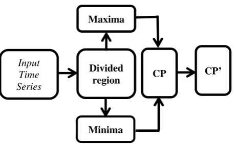
Figure 1. General Flowchart of the algorithm
A. FEFN Basics
Let {x[n],n=1,…,N*M} be an N*M time series which we will refer to as x[n].T is the time series of one whole experiment, Let { Ti, i=1,…,M} be an M-element time series which is the M equal segments. The value of M can affect the result of an operation, so we will discusses in detail in the subsequence sections. There are N elements in one segment. Let{(L[i],x[L[i]]),i=1,…,M} be an array with M elements which is maximum value in i segment. Let{(S[i],x[S[i]]),i=1,…,M} be an array with M elements which is minimum value in i segment.
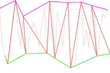
Maxima Envelope: The maxima envelope of a time series is Line segment passes through all of its maxima.(see the purpose one in Fig. 2)
Minima Envelope: The minima envelope of a time series is Line segment passes through all of its minima. (see the green one in Fig. 1)
M’value: The value of M is can affect the result of the maxima Envelope and the minima envelope. Polylines with the different M’s value are in Fig.2
Cross Polyline: Starting points and end points of the cross polyline come from the set of maxima Envelope and minima Envelope alternately. Firstly we take out a node from maxima envelope as the starting node, and take out a node from minima envelope as the end node, and drawing a straight line joining these two points. The end node from minima envelope becomes a start node, and end node is the second node in maxima envelope then. These nodes from maxima envelope and minima Envelope alternately are taken out and are joined together. The implementation process of joining lines is two steps. One is MaxtoMin line, the other is MintoMax line. Cross Polyline (CP) is the set of MaxtoMin and MintoMax. Tcp is the number of every segment as in (1), and fcp is reciprocal of Tcp as in (2).
Figure 2. Comparison between different value of M. For both (a) and (b), the red curve is original time series, and its superior and inferior envelopes are depicted as pink and green dashed curves. The value of M
in (a) is larger than in(b).
Tcp N/M (1) fcp M/N (2) Theoretically, we divide time series into M equal divisions. All data from CP curves are the maximum and minimum values which were selected from M parts. These data could present features of each part’s data. Each part is an independent part of data processing, and the interpolation operation will be implemented in each part at last. We could not retain all data in CP curves in solving practical problems. We need analysis data in CP curves, and eliminate data which could not present features of original data information. After the modification of CP’ curves could keep the primary data features using few data.
In short, the objective of algorithm is removing the noise data which disturbs data presenting, and forming CP curves which we defined after divided time series. With the relevant algorithms, some useful data was reserved, and useless data was removal. The improved CP’ curves instead of intrinsic curves
B. CP Process
The main process of FEFN forms CP curves and CP’ curves from time series data. Firstly, we divide time series into M region, and form CP curves. By analyzing the data of CP, We realize data removing and merging.
M’s value: the algorithm idea is choosing the maximum and minimum in every region, and presenting data character with these data. There are the maximum and minimum in every region, and connect these data to generate CP curves. Of course, there are some anomaly data in those data. The selection of extreme is greatly affected by the number of anomaly data. The method of removing anomaly data is removing several maximum and minimum, and the more accurate method is removing the middle node in three consecutive nodes which crossing angle is small. Yi-1, Yi, Yi+1 is value of three
consecutive nodes. Because of the same sample time, there are the same the abscissa value. The value is t0. We could calculate the angle α with Yi-1, Yi, Yi+1 and t0. If
the angle α is smaller than a given threshold, Yi is
considered as an anomaly data which we call noise data and will be removed. An approximate method used to find out noise data could be chosen .the value of
ΔYi/ΔYi+1or ΔYi+1/ΔYi is larger than a given threshold, Yi
is considered as an anomaly data as in (3) and (4). (b)
(a) Input Time Series
Divided region Maxima
Minima
ΔYi=|ΔYi-ΔYi-1| (3) ΔYi+1=|ΔYi+1-ΔYi| (4)
Figure 3. The positional relationship of the three consecutive points
We begin to define the value of M after removing noise data. The principle of selecting M’s value is satisfied with such conditions.
1. For the convenience of the interpolation operation, extreme value distribution in each region should be comparatively distributed with the mean distance. The distance between two consecutive maxima or minima should be close to Tcp. If we are able to determine the M’value with the basis of the analysis and comparison of previous data, its calculation efficiency is higher.
2. In the process of determining the value of M, it should try to ensure the maximum and minimum values appear alternately.
Because of data’s own characteristics, it is very difficult to meet the above requirements. If the value of M is the close to or meets the need of requirement, there is a high efficiency in the back of the computing process. The value of M should be greater than 1/2 of the cycle of changes in the value of the brain signal in general case. If the value of M is not larger than the cycle of the signal changes in the brain of 1/2, some data may be lost.
Figure 4. CP line
C. Interpolation&CP’ Process
After determining the value of M, We divide time series into M segments. Maximum value in each segment will be put into L[i], and minimum value will be put into S[i]. Variable iis the NO. of segment, and the values of i are chosen between 1 and M. under the perfect conditions, Connection of the data in the L and S may be formed CP.
In the three points, if there is a maximum near the point of maximum value, the subsequent far greater than a maximum value, we can remove the intermediate value.
Reducing the data in Lensure that this data does not exist in the L. The S array data is processed in the same way. In the CP of the maximum value and minimum value curve, we remove the peak around the protrusion, and the extreme point of attachment is retained.
After getting a simplified L and S array, we can select the value in turn. In the L and S data, the points will be connected into CP which meets the conditions. The method is that the maximum value point appears in the individual changes will be retained, and others points will be removed.
After getting the line which is simplified, we will form smooth curve with interpolation method. In the common interpolation algorithm, we can construct interpolation points according to the points we provided, and then formed a relatively smooth curve. But the interpolation curve can't meet our requirements. Because the interpolation data cannot guarantee form in accordance with the original discount trend, and it does not guarantee that the extreme we give is appeared in the curve peaks and troughs, as shown in Fig 5. Therefore, we need to improve the interpolation algorithm.
Figure 5. Interpolated curve
In the process of traditional interpolation algorithm, when the number of interpolation points and operations are too many, so the insertion value is uncertainty. It is said that although we can get the given value, there will be a great deviation between "fact" and the value in the vicinity, this kind of phenomenon is also called "the Runge phenomenon”. The solution is piecewise interpolation polynomial in low degree, to reduce the interpolation point. According to the features of the data we need interpolation, we need to be closed interval segmentation, to make the relatively small number of interpolation points in each cell and then to interpolate between each cell.
After determining the number of interpolation points, according to the experiment data, the effect between the two interpolation points in about 5 is relatively satisfactory, but more than 10 will be more serious, so if the interpolation points are not too many, every interval with 5 interpolations can get good effect. But to ensure that each contact more closely, make the interpolated curve more smooth, we should let the interval contains several identical interpolation point in the interval distribution .The number of selected the interpolation points for N, The interpolation points for each interval contains m.
Our approach is in accordance with the sliding window, Yi-1
Yi
Yi+1
α
the window contains the M points, each window sliding down the instrument point. This two time interpolation calculation of a point M-1 is repeated last used interpolation point. The algorithm only needs to compute at point N-m+1, the end of the computation. The smoothness of the m value determination will affect the curve.
In the interpolation process, we can obtain a smooth curve. However, the curve is not necessarily according to data changes. Drawing line graph we can use three points to finish a crest or trough description. But when we use the same three points to describe smooth curves, it is unable to draw the desired curve. Therefore we need to interpolate some supplemental point, which can guide the interpolation algorithm meet the requirements during the interpolation process. Derivation formulas are as in (5), (6) and (7).
∗
∗ . (5)
a0= (6)
a (7)
In order to obtain a smooth curve segments, we can define each segment as a parabola. Supposing a parabola through two points (x0,y0) and (x1,y1), we cannot
determine it pass through point (x2,y2).We can use the
similar point (x’2,y2) to replace point (x2,y2),and the
abscissa of (x’2,y2) is the same as abscissa of vertices
which could be calculated. According to the longitudinal coordinate the coordinates of two points and a point, we could get the coordinate of new vertices.
In the process of solving equations, we can get expressions for a and a0. We analyze that the auxiliary
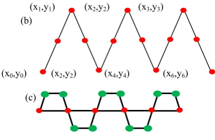
points have the effects on the procession of interpolation S. The five points we selected are assumed as the feature points. If we want the interpolated curve to pass through these five points, and these five points are continuous peaks of the curve, the curve will pass through the intermediate points of the connection of each two adjacent points. The intermediate points will be added into original peaks to calculate auxiliary points’ position. We use the auxiliary points to replace original the characteristic points to realize interpolation calculation. We find six intermediate points as characteristic points in the connectivity, and figure out 12 new points as the auxiliary points to complete the interpolation calculation (Fig. 6).
Figure 6. (a) is using (x2’,y2) to replace (x2,y2).Calculate new points
with (x0,y0), (x1,y1) and (x2’,y2).For both (b) and (c), the redpoints are
characteristic points, and the green points are auxiliary points.
Because the expression needs to prescribe in the calculation process, the a0 may appear two values in the
process of calculation. We can judge the two values which is consistent with our design curves. With analysis of the data, a0 is the abscissa of parabola apex, and it is
the value of the x2’. a0 value should be between x0 and x1.
In this way we can choose one of the two values as a curve equation of value. However, in different circumstances, every time we need to compare the relationship of three values to get the curve of a0 value.
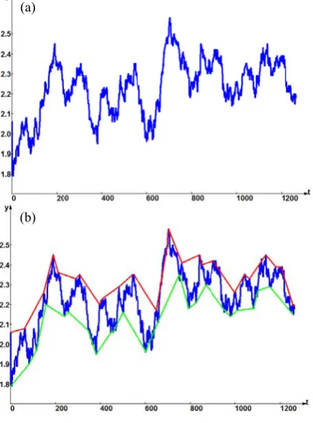
From the first set of data, we can see that there are large fluctuations in the original data curve. By analyzing the data, there is the difference result in brain surface oxygen concentration. In the continuous movement of finger case, there is larger fluctuation in the brain blood oxygen concentration. We hope that with the new method, the output of oxygen concentration curve is smooth.
III.RESULT
Ten experiments which have been popularly used in BCI are designed and implemented to revalue and validate the proposed ENDS. During these tasks simultaneous measurements of NIRS were performed. The NIRS-System was equipped with 37 optical fibers (15 sources with wavelengths of 850 nm and 760 nm, 22 detectors convolving to 37 measurement channels). Frontal, motor and parietal areas of the head were covered. The sampling frequency was fNIRS= 10 Hz. We choose 2 representative experiments with large fluctuations as the object we analysis.
The first study is based on non-continuous fingers motions on one side, and 20 sets of data of the sample divided into two groups which were selected as training set. The subjects were seated in a comfortable chair with armrests and were instructed to relax their arms. The experiment has 5 parts. Before the experiment, the subjects have 10 seconds’ rest. There are 20 seconds’ fingers motion and 30 seconds’ rest in every part. The subjects were finger movement on one side in each group. This enables us to situate the NIRS channel positions according to the standard 10 – 20 system.
(x0,y0) (x2,y2) (x4,y4) (x6,y6)
(x1,y1) (x2,y2) (x3,y3)
(b)
(c)
(x0,y0)
(x2,y2)
(x2’,y2)
(x1,y1)
Fig. 7(a) i large fluctua appeared. W we should d preliminary and the perio 50 data in ev we find out array and the Then the valu performance is minimum c According the points w curves, and 7(b).Based o "bulge" poin array and S minimum va and minimum
Through w original curv interpolation curve and th calculated va points CP1, four values interpolation values as the 7 (d) depict result betwee in Fig. 7(e). data reflect t changes smo
(a)
(b)
is a graph of ations betwee e start to proc determine the
analysis, the od of action i very group. W the maximum e minimum v ues of all L[i] curve. one is curve. g to the rules which need to remove the " on the two c nts, according array, we fin alue of the sing
m values are c we can see tha ve data from t n curve which he minimum alue in CP. Ac
CP2, CP3 in as the first n. We use the
e interpolation ts the interpo en original da According to the change tre ooth.
f the initial da en the second cess this data s value of M.
sampling fr is 20 seconds With 50 sample m value of eac value of a stor
] and S[i] are s maximum cu
defined abov o deal with "b "bulge" point, curves which
to the time nd the maxim gle direction, connected to fo at the basic ch
the CP line, i h can after a value, we n ccording to th
CP line, we c trapezoid us CPi-1, CPi, CP
n data, as show olation curve.
ata and the in the interpolat end of the dist
ata. There are d and third p set. In the first According to equency is 1 , so we deter e data in one g ch stored in t red into a S a connected to urve, and the o
ve, we should bulge" in the as shown in has removed sequence in t mum value and
and the maxim form CP in tur haracteristics o
in order to ge a maximum v need to inser he three contin could calculat sed to realize
Pi+1 to calcula
wn in Fig. 7(c) The compar nterpolation da
tion algorithm tance, and the
e two peaks t step o the 10Hz, rmine group, the L array. form other d find e two n Fig. d the the L d the mum rn. of the et the value rt the nuous te the e the ate f4 ).Fig. rative ata is m, the e data Figur orig as re curv W of tw two curv we trape Curv betw the o inter smo In phen featu whic seco
re 7. The proces ginal time series.(b ed and green dash
curve. Calculat ve.(d)Interpolation between
With the curve wo points on
points instea ve vertex with draw the pe ezoidal, and ve after inte ween the max
original data. rpolation base
oth curve. n the sec nomenon is ve ure points, we ch should be ond group data
(c)
(d)
(e)
ssing of the first g b)the superior and hed curves.(c)the c ted nodes are con n curve is depicte original data and
e equation, we both sides of ad of vertex, h interpolation eaks and val
realize interp erpolation do imum value a Finally we u ed on CP' of
ond experim ery common a e should distin repaired and a is shown in F
group of data.(a) nd inferior envelop
cp line is depicte nnected into the r ed as green curve d interpolation cu
e can calculat f the top poin it can depic n algorithm. T lleys with fo rpolation with oesn't exceed and the minim use CP ' to ins
f data eventu
ment data, and obvious. nguish betwee
not. The proc Fig. 8.
the blue curve is pes are depicted ed as blue dashed
ed dashed .(e)Composition urve.
te coordinates nt. With these ct the smooth That is to say, our points of h trapezoidal. d the range mum value of stead CP. The ually forms a
Figure 8. The p is original time
as red and green curve. Ca curve.(d)Interp bet (a) (b) (d) (c) (e)
processing of the series.(b)the supe n dashed curves.( alculated nodes a olation curve is d tween original da
e second group of erior and inferior (c)the cp line is d are connected into depicted as green ata and interpolati
f data.(a) the blue envelopes are de depicted as blue d o the red dashed curve.(e)Compo ion curve. e curve epicted dashed sition W that serie serie mini W extra gene inter info calle show in qu data coul main hem moti In FEF of th we calcu can extre of i inter The segm part extra the poin then com time guar auxi ensu ensu sour T Rob their also of L auth Dep
[1]
[2]
We presented iteratively e es data. The F es into some r imum value in With extreme action of ei erated CP cu rpolation is a
rmation, we u ed CP’ to repl w data curve b
ualitative agre a is in qualita ld output sta nly for test moglobin has
ion.
n this paper w FN framework
he data. Based represent the ulate the new
reflect the eme, it should interpolation. rpolation and new algor mentation, and . We extract act the maxim data points e nts. That is to n the initial d mputing, we on
e complexity rantee the ou iliary point t ure the data c ure the outpu rce data.
The authors botics Laborato
r support to c thank for the Liaoning Pro hors also tha partment of Lia
Flandrin, Patri decomposition International Information Pr M. Alamgir, M learning for
IV.CONCLU
a novel NIRS extracts the e FEFN framew regions and ex n every region e processing igenvalue of urves. In ord greement with use a group of
ace data of CP based on CP eement with o ative agreeme ble control s ing crowd greater fluc
we focused o k, and how to d on the maxim e variation ch
data point wi characteristics d be suitable
So the data it is suitable rithm is ba d the whole da characteristic mum value an
ach region ar say, if the da data will be r nly analysis 2 is reduced tput data is c to realize int
ontinuously a ut curve to r
ACKNOWLED
would like ory, Kochi Un conduct NIRS
e support of N ovince under nk for the s aoning Provin
REFEREN
ick, and Paulo ns as data-drive Journal of W rocessing, Vol. M. Grosse-Went Brain-Compute
USIONS
S data extract eigenvalue cu work divides th xtracts maxim n.
g, we imple f the origina rder to ensur th features of f calculated da P. The experim
' data after in original data. T ent with origi
signals. This ‘data whose ctuation with
on the presen o extract the f imum and min haracteristics ith the feature s to replace for interpolat a curve is sm
as a control ased on tim
ata is divided c values for e nd the minim re replaced by ata is divided
reduced to 2 2*M data, so substantially. continuous, w terpolation. N and smoothly, reflect the ch
DGMENT
to thank th niversity of Te S experiments
Natural scienc Grant 2013 support of th nce under Gra
NCES
Goncalves, “E ven wavelet-lik Wavelets, Multi 2, NO. 4. 2004 trup, and Y. Al ter Interfaces”
ion algorithm urves of time he whole time mum value and
emented the al data, and re data after f original data ata which was mental results nterpolation is The smoothed inal data, and algorithm is e oxygenated h continuous
ntation of the feature points nimum values of data. To e points which the original tion algorithm moother after signal output. me sequence into the same each part, and um value. So y two feature into M parts, *M times. In the algorithm In order to we design the Not only can , but also can hanges in the
he Intelligent echnology for . The authors ce Foundation 020032. The he Education nt L2011021. Empirical mode ke expansions”, resolution and 4, pp. 477-496.
Conferen (AISTAT [3] B. Blank Kübler, “Neuroph Performa 1303–130 [4] S. Fazli,
J. Steinbr a hybrid Image, V [5] T. Tsubo robot con infrared Internatio 26, 2007, [6] Daly, Jan interfaces Vol. 7, N [7] Fan Deng
Liu, “FM decompo engineeri [8] M. De Matthews define di human b 1359-136 [9] D. J. Hee neuronal 142–151, [10]N. K. Log
with fmri 2008. [11]G. Buzsk
cortical n 1929, Jun [12]Xiangjun
on W
Monitorin pp. 2686-[13]Xinming Method Algorithm of compu
nce on Artifi TS 2010), May kertz, C. Sanne K. R. Müller hysiological p ance”, Neuro Im
09.
J. Mehnert, G. rink, and B. Bla NIRS-EEG B Vol. 59, NO. 1, 2 one, T. Murog ntrol using bra spectroscopy”, onal Conferenc , pp. 542–534. nis J., and Jona s in neurologica NO. 11, 2008, pp g, Dajiang Zhu, MRI signal ana sition”, IEEE ing, Vol. 60, NO
Luca, C.F. B s, and S. M. Sm istinct modes o brain”, Neuroim 67.
eger and D. Re activity?”,Natu , Feb. 2002.
gothetis, “Wha i”, Nature, vol.
ki and A. Dr networks”, Scie n. 2004. n CHEN, Zhanf Wavelet Anal ngSystem”, Jou -2691.
Zhang, Lin Y Based on Ch m for Two-Dim uters, vol. 5, no.
icial Intelligen 13-15, 2010, pp elli, S. Halder, r, G. Curio, predictor of
mage, Vol. 51
Curio, A. Villr ankertz, “Enhan Brain Compute 2012, pp. 519-5 ga, and Y. Wa ain function me Proceedings o ce of the IEEE
athan R. Wolpa al rehabilitation p. 1032-1043. , JingleiLv, Lei alysis using em E transaction O. 1, January 20 Beckmann, N. mith, “fMRI re of long-distance mage, Vol. 29,
ess, “What doe ure Rev. Neuros
t we can do and . 453, no. 7197
raguhn, “Neuro ence, vol. 304,
feng GAO, “Da lysis in urnal of compu
Yan. A Fast I haos Optimizat mensional Tsal . 7, pp. 1054-10
nce and Stat p 17–24.
E. M. Hamme and T. Dick SMR-based , NO. 4, 2010
ringer, K.-R. M nced performan er Interface”, N 529.
ada, “Applicati easurement by of the 29th A
EMBS, Augus
w, “Brain–com n", Lancet neur
i Guo, and Tian mpirical mean
s on biome 013, pp. 42-54.
De Stefano, esting state netw
e interactions i , NO. 4, 2006
es fmri tell us sci , vol. 3, no.
d what we cann 7, pp. 869–878
onal oscillation no. 5679, pp. 1
ata Processing B Structure H uters, vol. 6, no
Image Thresho tion and Recu lis Entropy. Jo 061. tistics er, A. khaus, BCI 0, pp. Müller, nce by Neuro on to near-Annual st 23-mputer rology, nming curve edical P.M. works in the 6, pp. about 2, pp. not do , Jun. ns in 1926– Based Health o. 12, olding ursive ournal [14] [15] S. Waldert, Birbaumer, A. direction deco Neuroscience, Lebedev, Mik machine interf Neurosciences
H. Preissl, E Aertsen, and C oded from M
Vol. 28, NO. 4 hail A., and M faces: past, pres , Vol. 29, NO.
Yan Jiang
Institute o technology in 2009. C Professor Technology XML and in
Xin Jin re in Shenyan in 2010. Cu Shenyang Co., Ltd, mechanical network.
Xin Li rece
computer s Shenyang U 2013. Cur student at Technology and the data
E. Demandt, C. Mehring, “H MEG and EEG 4, 2008, pp. 100 Miguel AL Nic sent and future 9, 2008, pp. 53
received the P of information
from Northeas Currently, he is at Shenyang y, China. His i ntelligent contr
eceived the Bac ng University o urrently, he is Hexing Testin China. His in l control a
eived the bache science and tec University of rrently, she i t Shenyang y. Her interest a processing.
C. Braun, N. Hand movement G”, Journal of
00–1010. colelis, “Brain-e", TRENDS in
6-546.
Ph.D. degree in n science and stern University s an Associate University of interests are in rol.
chelor's degree of Technology, an Engineer at ng Equipment nterests are in and computer