Reduced Context Consistency Diagrams for
Resolving Inconsistent Data
Viktoriya Degeler
∗, Alexander Lazovik
Distributed Systems Group,
Johann Bernoulli Institute, University of Groningen, Nijenborgh 9, 9747 AG, The Netherlands
Abstract
The ability of pervasive context-aware systems to perform efficiently relies on their ability to gather full and unambiguous information about the environment. But raw data collected from sensors is often noisy, imprecise and corrupted, which leads to inconsistencies and conflicts in gathered data. Also environment is only partially observable, thus allowing ambiguities in the knowledge about its state. In the paper we present reduced context consistency diagrams (RCCD), data structures that allow to store the information about the environment even with the presence of inconsistencies, conflicts, and ambiguities. We provide a mechanism for reasoning about the current situation using these diagrams, and show how to obtain information about the most probable situation at each moment of time. The case study shows the 50% reduction in incorrect sensor readings. The evaluation shows RCCD to be applicable to real-time context inference problems.
Received on 21 July 2011; accepted on 5 November 2012; published on 26 November 2012
Keywords: Context-aware computing, context reasoning, context inconsistencies.
Copyright © 2012 Degeler and Lazovik, licensed to ICST. This is an open access article distributed under the terms of
the Creative Commons Attribution license (http://creativecommons.org/licenses/by/3.0/), which permits unlimited
use, distribution and reproduction in any medium so long as the original work is properly cited. doi:10.4108/trans.ubienv.2012.10-12.e2
1. Introduction
Pervasive context-aware systems become increasingly more complex and penetrate our daily life in forms of smart environments [13], context-aware applications on mobile devices, context aware autonomous systems, etc. The ability of such systems to perform efficiently fully relies on the ability to obtain the most detailed, specific, and correct information about the environment.
However, before high-level applications may use the information to make the appropriate decisions and adjust their behavior, several steps are required to obtain the information in a proper form. First of all, raw sensor readings should be gathered by a system’s middleware from surrounding sensors. Then they should be pre-processed, converted to a logical form, and combined together to obtain an image of the current environment. Afterwards the information should be converted to a form, understandable by a high-level application.
∗
Corresponding [email protected]
Unfortunately, several challenges arise during this process. The sensors are often noisy, imprecise, and their readings are easily corrupted, which may lead to inconsistencies and conflicts in gathered data. Also, the full information about the environment is practically impossible to obtain. Some portions of the environment can not be physically read by given technology, and there is always something happening that sensors miss to detect, e.g. the study by Jeffery et al. [12] showed that in dynamic environments the percentage of correctly read RFID tags may drop down to 60-70%. Another issue of sensor readings gathering is that information becomes obsolete rapidly. The data that was correct at the time of reading may be already obsolete when it reaches the system middleware and gets processed. The asynchronous nature of sensor readings leads to alterations in the order of readings arrival to the middleware. Finally, the automated processing of sensor readings to an interpretation of the environment may introduce errors by itself. The classical examples of such errors are image recognition mistakes.
one of the readings that is deemed as incorrect one based on some heuristic strategy. Different heuristics are proposed, among which the removal based on relative frequency [5], latest, oldest, drop-all, or drop-random [20] strategies.
Such a removal is usually done as soon as a conflicting sensor reading is received, to keep the full interpretation of an environment without conflicts. The removal of sensor readings in an ambiguous situation may, however, cause even more problems, in case the correct sensor reading is removed instead of an incorrect one. The more cautious approach that removes all conflicting sensor readings, may drastically reduce the available amount of information, which is used by high-level applications to make decisions.
In [6] we introduced originally context consistency diagrams (CCD), which are capable of storing all gathered information, and define several possible context interpretations in a presence of a conflict or an ambiguity, either because of incomplete knowledge about the environment, or because of erroneous sensor readings. If all the information is kept, further sensor readings help to refine the knowledge and make more informed decisions about the correctness of certain sensor readings. In this paper we extend a notion of CCD and introduce a reduced context consistency diagram (RCCD) for dealing with inconsistent and incomplete data, which severely reduces the resulting diagram size comparing to the original full CCD. The CCD and RCCD are capable of storing all the information without discarding anything, even if the data has conflicts. RCCD, while having a less extensive querying capabilities than CCD, requires much less computational and storage power. Pervasive systems can implement either CCD or RCCD mechanism to deal with ambiguous or conflicting context data.
The rest of the paper is organized as follows. Section2 overviews a proposed architecture of a context-aware system with implemented CCD or RCCD functionality. In Section 3 we formally define environment and an information about it in a form of different contexts. Section 4 introduces CCD. RCCDs are introduced in Section5, and their respective maintenance is described in Section 6. Section 7 shows querying capabilities of RCCD, and describes a way to obtain useful information about the state of environment out of them. In Section8 we present some complexity considerations over CCD and RCCD, and in Section 9 we perform a case study and evaluate performance of RCCD. Section10 discusses the related work. Finally, in Section 11 we provide our concluding remarks.
2. System overview
In this section we describe a system that collects raw sensor readings and interprets them to create an
Figure 1. Context reasoning using CCD.
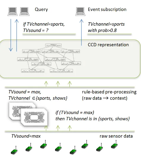
image of the environment. A high-level overview of the proposed system architecture is shown in Figure1.
At the bottom level the sensors read the state of certain entities and pass it to the system’s middle-ware. Readings can be of different nature, with the most common being a stream of ‘variable=value’ pairs, for exampleT V channel=sports. Also ranges of values can be given, if a sensor is imprecise. After the system obtains this raw sensor data, a rule-based pre-processing is performed. The rules define the interdependence of variable among each other, and the limitations that one variable value puts on other variables. The pre-processing transforms a raw data into a context information. For example, as shown in Figure1, a rule (T V sound=max =⇒ T V channel∈ {sports, shows}) is applied to a sensed value (T V sound=
max). The resulting pre-processed context (T V sound=
sensor or by data expiration should not stop the sys-tem from providing the best possible interpretation for the acquired context information. Several techniques exist to resolve an ambiguous conflict in favor of one interpretation. But if the resolution is incorrect, further interpretations of a situation will also be wrong, even if further information may show that another solution was preferable.
To deal with this, CCD keeps several interpretations, each with its own probability of being true. We associate a likelihood of being true to each acquired chunk of data. Whenever chunks “support” each other (there is an interpretation of a situation that is consistent with all of them), their mutual truth likelihood is higher comparing to the conflicting ones. Additionally, each arrived and pre-processed information shares a certain degree of truth likelihood, thus compensating the effect of a faulty sensor over the inferred information received from that particular sensor. The most probable interpretation is then the one that is “supported” by the majority of consistent contexts. Even if a particular context does not support the most “popular” interpretation, it is still stored in a CCD. It might happen that with the acquisition of new data, the context is considered more likely, if the new data supports it. With such a structure the context interpretation is never final, as new data may change the interpretation by contributing to an interpretation previously considered wrong.
High-level applications can use CCD layer for obtaining different information about the environment. One of such possible usages is querying. Among the queries that CCD supports are “What is the most probable situation at this moment of time?”, “What are the probable values of a certain variable?” (For example, in Figure1: “What are probable values of TV channel?”), “Assuming certain additional information, what are the probable values of a certain variable?” (For example, “Assuming TV channel is ‘sports’, what is the probability distribution of TV sound values?”), etc.
Another possible usage of CCD layer is event subscription, which commonly appears in a form “Notify as soon as a certain situation happens with a certain probability.” (For example, “Notify in case TV channel is ‘sports’ with probability more than 0.8.”)
3. Environment and context
A server that collects raw data (pre-processing layer in Figure 1) obtains information from the underlying layer in a form vi =dij, i.e., a variable vi has a value
dij. It is possible that the sensors return a set of values, i.e.,vi ∈ {dij
1, dij2}. For example, a location variable may
be sensed by a sensor (e.g. RFID) that is known to be imprecise.
Definition 1 (Environment).An environment hV , Di is defined by a set of context variables V = {v1, v2, ..., vn}. Each variable vi varies over a domain
Di ={di1, di2, ..., dim
i}with sizemi.
Many variables either cannot be directly observed, or can only be partially sensed. If the heating mechanism is broken, we can sense that the heater is turned on, but we cannot observe if it actually started to heat the room, unless we have a reliable temperature sensor. Fortunately, many variables influence each other. For example, it is impossible to have a light turned on, if there is no electricity in the house; a location of a person and of the tool that she works with must be the same, etc. If these correlations are taken into account, even a few observed variables may give an overall, yet possibly incomplete, knowledge about the environment.
Definition 2 (Context, Interpretation).For a given environ-ment hV , Di, a context c is a valuation of all variables inV with a non-empty subsetDcofD. If all variables
vi are assigned one and only one specific value inDi, a
context is called aninterpretation.
Non-emptiness ensures that a context is always possible in practice, i.e. each variable has at least one possible value.
We represent a context by enumerating its possible context variables values:D0c, . . . , Dnc, or, alternatively, as
v0∈ {d0l, . . . , d0k}. We writec.vi to refer toi-th variable
of contextc.
Our knowledge about an environment is described by a set of contextsc0, . . . , cn. If for any two interpretations x, ys.t.∀ci :x∈ci∧y∈ci, it follows thatx=y, then we have complete and unambiguous knowledge about the given environment.
More than one interpretation represents an ambi-guity or incomplete knowledge of the environment. Intuitively, each new sensor reading adds some more knowledge about the environment, thus it reduces the number of possible interpretations. Faulty contexts can be detected when an impossible situation is created, i.e. when there is no interpretationx, s.t.∀ci :x∈ci.
Table 1. Example of environment and context creation.
(a)Variables.
Variable Domain
Electricity off, on Light off, on
TV off, news, sports, shows TV sound 0, 1, 2, 3
(b)Dependency rules.
¬(E=of f∧ Light and TV can be turned on (L=on∨ ¬(T V =of f))) only if electricity is on.
¬(T V =of f∧ Non-silent TV sound means
T V s∈ {1,2,3}) TV is turned on.
T V =shows⇒L=of f If TV channel is ‘shows’, light should be turned off.
(c)Sensor readings and contexts.
ID Sensor reading Context
c1 T V =Sh E: 1|L: 0|T V :Sh|T V s: 0123
c2 T V s= 2 E: 1|L: 01|T V :N SpSh|T V s: 2
c3 L= 1 E: 1|L: 1|T V : 0N Sp|T V s: 0123
c4 T V ∈ {Sp, Sh} E: 1|L: 01|T V :SpSh|T V s: 0123
A set of contexts C ={ck} is consistent if there exist at least one interpretation x:x.vi =diji,∀i∈1..n such that diji ∈ck.vi, ∀ck ∈C, ∀i∈1..n. A set of contexts is
inconsistentotherwise.
Additionally, we define two relations over contexts:
Inclusion:c1⊂c2 iff ∀i∈1..n: c1.vi ⊂c2.vi Inclusion
can be viewed as a relation of a more precise and less precise contexts. Ifc1⊂c2 then contextc1 is more
precise, than c2, in other words, each variable of c1
contains less values that are possible.
Intersection:cu =Tk
j=1cj =c1∩c2...∩ck iff∀i∈1..n:
cu.vi =c1.vi ∩c2.vi...∩ck.vi An intersection of
inconsis-tent contexts always equals to ∅. An intersection of
consistent contexts is a context, that is at least as precise, that any of the originals:∀j∈1..k cu ⊆cj.
4. Context consistency diagram
To compactly represent all possible interpretations for a given set of contexts, we use relations defined in the previous section, thus forming a diagram with arrows representing inclusion relation. Any two contextsci, cj
are connected in the diagram, ifci ⊂cj, and there is no
suchck, so thatci ⊂ck ⊂cj.
The idea of putting contexts into the diagram structure is essentially an introduction of a compact representation of all possible interpretations of the environment. The “full domain” context is always at the top, meaning “no information is received; any situation is possible.” Starting from the top and going down, contexts become more and more restrictive, with the most restrictive (as well as the most knowledgeable) contexts at the bottom. Formally, CCD is defined as follows:
Definition 3 (Context consistency diagram (CCD)).Given an environmenthV , Diand a set of contextsC0={ck}, k∈
Figure 2. Example of context consistency diagrams.
1..N, acontext consistency diagram (CCD)is a tupleG= hC, E, ri, where:
• r=D, is a special context, theroot;
• C=C0∪Cu∪r where Cu is the full set of
intersections of a power set ofC0;
• E⊆C×C, such that (c2, c1)∈E iff ∃c1, c2∈C:
Contexts from a setCare vertices of the diagram and
Eis a set of directed edges. In a relationship (c1, c2)∈E,
c1 is called a parent, and c2 is called a child. cp is
called apredecessorofcc, and, respectively,ccis called adescendantofcpif either of the following holds:
1. (cp, cc)∈E
2. ∃{ci} ∈C, i∈1..k s.t.(cp, c1)∈E∧(ck, cc)∈
E∧(ci, ci+1)∈E,∀i∈1..k−1
We writeψ(c) to denote the full set of descendants ofc
andΨ(c) to denote the full set of predecessors ofc. For a set C0={c1, c2, c3}, the corresponding set of
intersections of its power set is equal to Cu ={c1∩
c2, c1∩c3, c2∩c3, c1∩c2∩c3}.
For a set of contexts listed in Table 1c the corresponding CCD is shown on Figure2.
In [6] we describe in details the characteristics of the CCD, its properties, and algorithms for maintaining the CCD in real time.
5. Reduced context consistency diagram
While CCD provides a full picture of the information together with existing inconsistencies, it is a verbose structure that shows all the possibilities of environment knowledge explicitly, thus at the expence of computa-tional and storage power.
For this we devised the way to reduce a classic CCD, while still keeping the knowledge about existing inconsistencies intact. The reduced context consistency diagram (RCCD) uses the fact that some of those nodes that are not received from sensor readings, but are created as intermediate ones, are combined together to create a more knowledgeable common descendant. If this is the case, those intermediate nodes can be truncated from the diagram, while still keeping the information about the most probable situation.
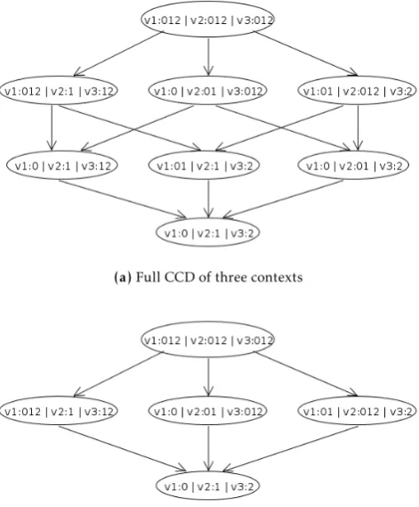
For example, in the case, described in Figure3aa full CCD is shown for the following three contexts:
c1= (v1∈(0,1,2); v2= 1; v3∈(1,2))
c2= (v1= 0; v2∈(0,1); v3∈(0,1,2))
c3= (v1∈(0,1); v2∈(0,1,2); v3= 2)
However, the three generated nodes of the second tier can be reduced, as they all are combined in the more knowledgeable context (v1= 0; v2= 1; v3= 2). The
corresponding reduced CCD is shown in Figure3b. Notice that the RCCD may reduce only nodes that were not originally obtained from sensor readings (in other words, those nodes that do not belong toC0group
and do not have associated initial weightw0(c)). In the
same example, the full CCD will be exactly the same as reduced CCD (both as shown in Figure3a) in case we also receive three more sensor readings that account for
(a)Full CCD of three contexts
(b)Reduced CCD of the same contexts
Figure 3. Example of a full CCD (a) and a corresponding reduced
CCD (b)
the following contexts:
c4= (v1= 0; v2 = 1; v3∈(1,2))
c5= (v1∈(0,1); v2= 1; v3= 2)
c6= (v1= 0; v2 ∈(0,1); v3= 2)
The formal definition of RCCD goes as follows:
Definition 4 (Reduced context consistency diagram (RCCD)).
Given an environment hV , Di and a set of contexts
C0 ={ck}, k ∈1..N, areduced context consistency diagram
(RCCD)is a tupleGr =hC, E, ri, where:
• r=D, is a special context, theroot;
• C=C0∪Cr∪rwhereCris defined asCr =Scp∈
Cu\(C0∪r)s.t.@cc∈Cu∪C0: (cc⊂cp))
• E⊆C×C, such that (c2, c1)∈E iff ∃c1, c2∈C:
c1⊂c2and@cm∈C:c1⊂cm⊂c2.
The only difference with the Definition 3 of CCD is the definition of a context set C, which, however, drastically changes the resulting diagram.
and all contexts out of the original context setC0.
Non-solidcontextsCnsare all the contexts out of a full set of intersection of a power setCuthat are not included into a solid set (thus that are not among original contexts).
Cs=C0∪r (1)
Cns=C\Cs (2)
As in CCD, vertices of the RCCD include all the solid contexts. However, unlike in CCD, where all non-solid contexts are also kept, in RCCD they are kept in the diagram only in case they are the most knowledgeable contexts.
This leads us to the first property of the RCCD:
Property 1.All non-solid nodes of RCCD do not have children.
Proof. If a nodec∈Chas a child, then by the definition of a context set C, this node may not be the part of Cr, because ∀c∈Cr:@cc∈Cu∪C0: (cc⊂c)). From facts thatC =C0∪Cr∪r, andc∈C, butc<Cr, follows
that c∈C0∪r, and by definition of a solid node from equation1,cmust be solid. Thus if a node of RCCD has a child, it is always a solid node. Thus non-solid nodes do not have children.
The second property of RCCD is:
Property 2.If all nodes with children of a full CCD are part of the original context setC0, then a corresponding
reduced CCD is equal to the full CCD.
Proof. Solid nodesC0∪r are always part of both CCD
and RCCD context sets, thus only non-solid nodes differ. We are given that all nodes of CCD with children are inC0set, thus for the remaining nodes the following
holds:
∀c∈Cu\(C0∪r) :@cc∈Cu∪C0: (cc⊂c))
which is exactly the definition of correspondingCrfrom RCCD. So
∀c∈Cu\(C0∪r) :c∈Cr
or
Cu\(C0∪r) =Cr
Thus,
Cf ull =Cu∪C0∪r= (Cu\(C0∪r))∪C0∪r=
=Cr∪C0∪r=Creduced
The fact thatCf ull =Creducedalso means thatEf ull =
Ereduced by definition of edges construction. So CCD and RCCD under the given conditions are equal.
All the original properties of CCD also hold for RCCD. Those are:
Property 3.For a given set of contexts there is one and only one non-isomorphic representation of its RCCD.
Property 4.The order of contexts addition does not change the resulting RCCD.
Property 5.Adding and then removing a context does not change the resulting RCCD.
The proof of these three properties for RCCD is exactly the same as for CCD and is presented in [6].
6. RCCD maintenance
In this section we present algorithms to add and remove a context to the RCCD.
Algorithm 1Adding context to RCCD
1: functionAddContext(context, parent, weight)
2: if∃ch∈parent.children s.t. ch=contextthen 3: W0(ch)←W0(ch) +weight
4: exit
5: else if ∃child∈parent.children.nonsolid s.t.
context⊂childthen
6: ∀child:Move parents fromchildtocontext 7: else if∃child∈parent.children.solid s.t.context⊂
childthen
8: ∀child:AddContext(context, child, weight) 9: else
10: CheckChildren(context, parent)
11: Add link fromparenttocontext
12: end if
13:
14: functionCheckChildren(context, node):boolean
15: result←f alse
16: for allchild ∈node.childrendo 17: ifchild ⊂contextthen
18: ifnodeis a parent ofcontextthen
19: Remove link fromnodetochild
20: end if
21: Addchildtocontextas descendant
22: result←true
23: else ifisConsistent(context, child)then 24: x←context∩child
25: if¬isSolid(child)then
26: Move parents fromchildtox
27: Add link fromcontexttox
28: result←true
29: else if¬CheckChildren(context, child)then
30: Add link fromcontexttox
31: Add link fromchildtox
32: end if
33: end if
34: end for
35: return result
AddContext recursively searches predecessors of the
context to find its parents, i.e. contexts, to which the new context should be added as a child. As soon as those parents are found, the second part, CheckChildren, recursively checks if a context is consistent with its brothers, and a child should be generated.
The first part, AddContext, checks if a parent is a parent of a context. It starts by checking if there is a child of aparent, equal to thecontext. If this is the case, a corresponding weight is added to the initial weight of a child, and algorithm finishes its work.
Otherwise it checks, if there are any non-solid children of a parent that are more general, than a
context. In this case all the parents of such children are moved and become parents of acontext. Note that this effectively deletes those children from the diagram, because they do not have parents anymore and non-solid nodes never have their own children.
If no suitable children are found yet, the algorithm checks, if there are solid children of a parent that are more general than acontext. In case they are found, the algorithm repeats recursively for them.
Otherwise we found a parent of a context. Second part of the algorithm, CheckChildren, is then called, and aparentadds acontextas a child.
CheckChildrenfunction receives two nodes as input, acontext, which is a newly added to the diagram node, and anothernode, for which we suspect that its children may be consistent with a context. We process all the children of thenodein the following manner:
If a child is included into a context, we add it as a descendant to acontext, and remove it as a child from
node, in case acontextis already a child of anode. Otherwise we check for consistency of acontextand a
child. If they are consistent, and achildis non-solid, we remove it from the diagram, and put an intersection of achildandcontextin its place. We also add a link from acontextto the new node.
If a child is solid, however, we check, if there is already (or should be created) a common descendant between achildand acontextby callingCheckChildren
recursively on those nodes. If it returns negative result, we add a new node (their intersection) to the diagram, by adding it as a child to acontextand achild.
Algorithm 2 describes the removal of an outdated context from RCCD.
First of all, the context can only be removed in case the context becomes non-solid after reducing the initial weight by the amount, corresponding to the outdated sensor reading. I.e. in case there are no more other sensor readings that support this context.
If acontexthas children, we first remove a link from context parents to it, and than add links from context parents to its children, connecting them directly.
After this, on lines 14-20 we check non-solid children of a context, or a context itself in the absence of
Algorithm 2Removing context from RCCD
1: functionRemoveContext(context, weight)
2: W0(context) =W0(context)−weight 3: ifW0(context) = 0then
4: ifcontexthas childrenthen
5: for allparent ∈context.parentsdo
6: Remove link fromparenttocontext
7: Add allcontext.childrentoparentas descen-dants
8: end for
9: nodes←context.children.nonsolid
10: Remove links fromcontextto all itschildren
11: else
12: nodes←context
13: end if
14: for allnode←nodesdo
15: x←T
node.parents
16: if x,node&@brth∈node.brothers s.t. brth⊂
xthen
17: Add link from allnode.parentstox
18: Remove links from allnode.parentstonode
19: end if
20: end for
21: end if
children, for the maximum generality. That means that each suchnodeshould stay on the diagram only if it still has more than one parent, and if the intersection of all its current parents is exactly equal to anode. It may be the case that after the removal of a parent, a non-solid
nodeis now less general, than it should be. In this case we create a new nodex, which is the intersection of all its current parents, and move all the parents of anode
tox, effectively removing anodefrom the diagram.
7. RCCD reasoning
own weight, only those interpretations of a parent that are also contained in a child gain this additional weight. Which by itself means that they become more probable, than the others. So, we proved that the interpretations, contained in a child, will always be more probable, than interpretations of a parent, which are not contained in any of its children. Which means that the most probable interpretation of a situation is always the one among nodes with no children.
RCCD by the definition4 never reduces nodes that do not have children, so they are always present on a diagram. Moreover, all the initial weights from original contexts are also transferred to these nodes, and all the consistency among original nodes is kept, as the way of inheriting nodes in RCCD is the same, as in CCD. Due to these facts the most probable interpretation has the biggest weight among all interpretations. The probability calculation, presented in [6] still can be used in RCCD for finding the most probable interpretation.
As well as CCD, RCCD never discards any informa-tion from sensors, and if the most probable interpre-tation changes with the arrival of a new context, the RCCD immediately catches this change.
7.1. Unfolding of RCCD to CCD
The previous subsection shows that for systems that are mostly concerned with a question “What is the most probable situation at this moment of time?” the RCCD is a more preferable choice of a diagram, than CCD. However, even for such systems sometimes there are cases when additional information about other possible situations or conditional probabilities are important to know. Fortunately, the choice of RCCD over CCD does not permanently hinders the ability to obtain the answers to these queries. We present an Algorithm 3 that allows to unfold a RCCD to obtain a full CCD.
The function U nf oldN ode will be called for every node of the diagram. At the beginning of the algorithm the queue contains all the most knowledgeable nodes (described byRCCD.lastnodes), i.e. nodes that do not have children. In other words, the algorithm unfolds nodes from the bottom to the top. The last node to be unfolded is always theroot.
U nf oldN ode is called either for all, or for a subset of node parents. When a node is polled from aqueue, the function is always called for all node parents, but later it can be recursively called for a subset of them. The function checks if there is only one parent among the inputparents. If it is the case, it checks, if all the children of a parent are already marked, and if it is the case, it adds a parent to the queue. If there are more than one parent in parents subset, the function tries to remove a single parent from this subset one by one, and checks, if the remaining parents can create a more general consistent childx, than anode. If it is the case,
Algorithm 3Unfold RCCD to CCD
1: functionUnfoldRCCD
2: queue←RCCD.lastnodes
3: whilequeueis not emptydo
4: node←queue.poll()
5: UnfoldNode(node, node.parents)
6: end while
7:
8: functionUnfoldNode(node,parents)
9: Marknode
10: ifparents.size= 1then
11: ifparents(0).childrenare markedthen
12: queue.add(parents(0))
13: else
14: for allpar ∈parentsdo
15: x←T
(parents\par)
16: ifx,nodethen
17: for allparent∈parents\pardo
18: Remove link fromparenttonode
19: for allchild∈parent.childrendo
20: ifchild⊂xthen
21: Remove link fromparenttochild
22: Add link fromxtochild
23: else ifisConsistent(x, child)then
24: y ←x∩child
25: Addyas descendant tochild
26: Add link fromxtoy
27: end if
28: end for
29: Add link fromparenttox
30: end for
31: Add link fromxtonode
32: queue.add(x)
33: else
34: UnfoldNode(node,parents\par))
35: end if
36: end for
37: end if
38: end if
the link from all such parents to thenodeis removed, and x is added as a child to them instead. Also each parent checks, if it has other children that either should now be the children of x (in this case the link from
parent to child is removed, and a link fromxtochild
is added instead), or that have a consistent childywith
x(y is than added as descendant to bothchildandxin this case). After this is done, the link fromxtonodeis added, and a new nodexis put to the queue.
8. CCD vs RCCD complexity
However, there are several considerations that help to keep the size of a CCD reasonable.
The biggest growth of a CCD results from faulty contexts. While correct contexts tend to have the same descendants, faulty contexts will generate many new CCD nodes. With a growth of a CCD, one may discard contexts that support the most unlikely interpretations, as most probably they represent faulty or imprecise sensors.
Each environment in a CCD should only contain interdependent variables (i.e. associated by dependency rules, as in Table1b). We split independent variables on non-intersecting subgroups and produce a smaller CCD for each subgroup.
RCCD, on the other hand, produces a much smaller diagram. First of all, notice that RCCD does not generate new nodes, unless they are the most knowledgeable. In case all the contexts are correct, the maximum number of nodes in RCCD will be Nc+ 2,
whereNcis the number of distinct nodes in the original
context set, and the number 2 corresponds to theroot
and a possibly generated single child. The child is single, because if all contexts are correct, they are all consistent with each other, thus they all have the same the most knowledgeable descendant.
Each erroneous context potentially adds Nv new children (alternative “most knowledgeable” nodes), one per each variable, where Nv is the number of
variables. Thus with the presence of erroneous contexts the maximum number of nodes in RCCD is equal to
Nc+Nv∗Nerr+ 2, where Nerr - number of erroneous
contexts. Notice that normally we assume a situation, whereNerr Nc, thus we expect small sizes of RCCD
in practice. If this is not the case, with bigger numbers of errors the RCCD size will grow as well.
9. Evaluation
Our evaluation section is split on two parts. First, in Section 9.1 we show a sample run of the system and discuss it in details. Second, in Section 9.2 we make a general overview of system’s performance based on several experiments, and study the dependence of system’s performance on different system parameters.
9.1. Case study
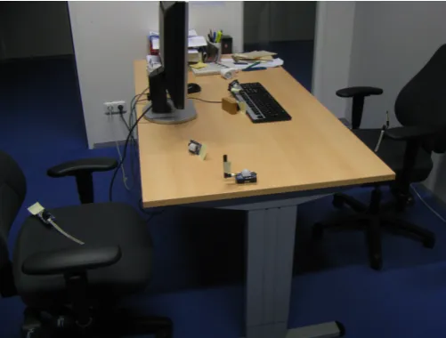
To evaluate the system in real conditions we performed an experiment with several sensors. The setup of the experiment can be seen in Figure4.
We used six sensors altogether: 2 acoustic sensors, 2 PIR motion sensors, and 2 pressure sensors. The sensors are produced by Advantic Systems [1]. They are IEEE 802.15.4 compliant wireless sensors that use open-source “TelosB” platform [17]. All sensors are equipped with ultra low-power 16bit microcontroller
(a)General view on the experimental place.
(b)Acoustic and PIR motion sensors.
(c)Pressure sensor.
MSP430. The pressure sensor uses the Tekscan® A201-100 FlexiForce® sensor, which provides force and load measurements for both static and dynamic forces (up to 100lb or 400N). The Passive InfraRed (PIR) motion sensor uses the Perkin Elmer Optoelectronics® LHI878 sensor to detect motion in the given direction. The SE1000 acoustic sensor has a mini-microphone (20-16000 Hz, SNR 58 dB) that is designed to detect the presence of sound. All sensors were configured to measure intensity of corresponding signals and thresholds were applied to readouts of each sensor in order to return a higher-level boolean value (presence or absence of sound/motion/pressure) once every second. The data was then sent to the RCCD structure, which in turn returned the current most probable situation.
Figure4ashows the general placement of the sensors. The setup shows the office of a single person and the idea of using such sensors is to be able to recognize a current activity of a person. Among those activities we assume work with or without PC, meeting with another person, or absence from the working desk. While each of sensors occasionally produces faulty readings, their mutual dependencies that we described in terms of rules, help RCCD to recognize the correct situation.
First we describe, what each sensor is aimed to recog-nize, then we describe their mutual interdependecies, and afterwards we will show the results of the experi-mental run of such a system.
Sensors description. Pressure sensor 1 (P R1)is located
on a chair of the main person in front of the PC, and is triggered if someone is sitting on this chair.
Pressure sensor 2 (P R2)is located on a “guest” chair,
and is triggered if someone is sitting on it.
Acoustic sensor 1 (AC1)is placed near the keyboard
and is aimed to detect the sound of keys pressing, in order to recognize the typing activity.
Acoustic sensor 2 (AC2)is a general acoustic sensor
that is aimed to recognize a sound in a room. It is placed in between the two chairs, because the sound usually means the conversation between the two people.
We want to note that keyboard typing, while triggering sound recognition onAC1, is not loud enough
to trigger sound recognition onAC2, thusAC2 remains
silent in this case. However, when two people are speaking with each other, both acoustic sensors detect sound. So we can only definitely recognize the keyboard typing whenAC2is silent, whileAC1is detecting sound.
PIR motion sensor 1 (M1)is directed exactly at the
front of the PC (looking directly at the first chair), and is aimed to detect any motion in this direction. The sensor gives us additional source of information, and can help to recognize the innacuracies of other relevant sensors.
PIR motion sensor 2 (M2)is looking directly at the
guest chair, and is aimed to detect any motion on or around this chair. This sensor as well gives us additional
source of information, and can help to recognize the innacuracies of other relevant sensors.
Interdependencies rules. As already noted, sensors in our case study have common dependencies. For example, when AC2 is detecting sound, AC1 is also detecting
sound (but not the other way around). When a person is sitting in a chair, both pressureP R1 and motionM1
sensors will detect activity. These and other dependies we capture by creating the following rules:
“Pressure implies motion.”Both motion sensors are
directed exactly on the chairs, and located very closely to it. When someone is sitting on a chair, in most cases the motion sensors detect small motions of a person in it. We help our system to detect the faulty readings of no motion by adding these two rules:
P R1 =⇒ M1 (3)
P R2 =⇒ M2 (4)
“Who is typing, if no one is there?” If we detect
no motion, and no pressure from the chair in front of the PC, and there is no general sound in the room, the keyboard acoustic sensor should also remain silent. Thus the third rule:
¬P R1∧ ¬M1∧ ¬AC2 =⇒ ¬AC1 (5)
Note that given the rule3, we can cancel out the variable
P R1 from this formula. However, we prefer to keep
it in this format both for ostensive purposes and for each rule to remain completely independent from other rules.
“I heard something. Did you hear it?” The first
acoustic sensor is placed very close to keyboard in order to detect soft noise of keyboard typing, which second sensor is unable to detect. The second sensor, however, placed just in the middle of the meeting area, in order to detect all loud noises in the room, the most common noise being human speech. The first sensor is able to detect all those loud noises also, which means it should always be triggered when the second acoustic sensor detects something:
AC2 =⇒ AC1 (6)
“Room is busy.” If we detect sound on keyboard
acoustic sensor, and a motion in general area, but not on the chair in front of the PC, it means the sound comes from somewhere else in the room, so the second acoustic sensor should also be able to detect it.
AC1∧M2∧ ¬M1 =⇒ AC2 (7)
Table 2. Experiment results
Sensor Number of errors Error rate,% % of errors fixed
Latest Averaged RCCD Latest Averaged RCCD Latest Averaged RCCD
M1 631 563 77 35.06 31.28 4.28 0.0 10.78 87.80
PR1 270 259 274 15.00 14.39 15.22 0.0 4.07 -1.48
AC1 398 336 314 22.11 18.67 17.44 0.0 15.58 21.11
M2 132 116 11 7.33 6.44 0.61 0.0 12.12 91.67
PR2 18 8 9 1.00 0.44 0.50 0.0 55.56 50.00
AC2 160 126 123 8.89 7.00 6.83 0.0 21.25 23.13
Total 1609 1408 808 14.90 13.04 7.48 0.0 12.49 49.78
1. For the first 10 minutes the person was working with the computer. Thus the expected correct values of sensors would be:
M1 =true; P R1=true; AC1=true;
M2 =f alse; P R2=f alse; AC2=f alse
2. Then the short meeting with another person was held for 5 minutes. The expected values are:
M1 =true; P R1=true; AC1=true;
M2 =true; P R2=true; AC2=true
3. After this the person was reading papers silently for 10 minutes. Corresponding expected sensor values:
M1 =true; P R1=true; AC1=f alse;
M2 =f alse; P R2=f alse; AC2=f alse
4. Last 5 minutes the room was empty:
M1 =f alse; P R1=f alse; AC1=f alse;
M2 =f alse; P R2=f alse; AC2=f alse
Results. Now we present the results that we obtained from the run. The experiment was running for 30 minutes, with sensors sending their readings each second. The lifetime of sensor readings is set to 5 seconds, so for each sensor we have 5 latest readings that are still to be considered. This is done in order to smooth the readings, as many sensors occasionally return incorrect readings (e.g. for a motion sensor it is common to return sequences such as “1; 2868; 2852; 1; 1; 2861; 2853”, where high values indicate movement, and 1 indicates no movement).
We compared the results of three possible sensors interpretations: first interpretation always takes the latest sensor reading and considers it correct; second one takes all readings with valid lifetime and chooses the most common (average) value; third one uses RCCD in order to find the expected correct sensor readings.
The results can be seen in Table 2. All sensors were returning faulty readings from time to time, with M1 sensor being the least reliable (35% of erroneous readings), and PR2 sensor being the most reliable with only 1% of readings being erroneous. While averaging
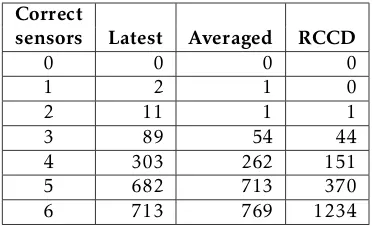
Table 3. Times seen each number of correct sensors
Correct
sensors Latest Averaged RCCD
0 0 0 0
1 2 1 0
2 11 1 1
3 89 54 44
4 303 262 151
5 682 713 370
6 713 769 1234
the value of sensors over their lifetime helped to reduce a number of erroneous sensors reading by 12.49%, the usage of RCCD to get the most probable situation reduced the number of errors for 49.78%, going from 1609 total erroroneous readings, to just 808.
Figure 5. Dependence of update time on number of sensors.
9.2. Performance
In this chapter we describe, how the system’s performance depends on parameters of a system. The experiments are performed on a Intel Core2Duo P7370 2GHz PC with 3 GB RAM running OS Ubuntu 10.04. The software is written in Java JDK 1.6. The simulated test environment consists of a test generation part that generates situation and contexts, and a middleware part that collects contexts and maintains a diagram.
The most important among all the parameters is the size of an environment, which is described by a number of sensors, or variables. We performed several experiments with the same parameters, while varying the number of sensors. The context arrival rate is set to 0.01 seconds; context lifetime is set to 4 seconds in the first experiment, and 6 seconds in the second. The test generation part creates a situation. Contexts are generated based on it with a 5% error rate and are sent to the middleware part. The results can be seen in Figure 5. As can be seen in this figure, the average time needed to update a RCCD with each new context increases linearly with the increasing of sensors number, until it reaches some point (in this case 700 variables), after which the time remains on a same level. This can be explained by a fact that while environments are relatively small, the increase in the environment size leads to an increase in RCCD number of nodes. However, for a certain context arrival rate and a certain context lifetime there is a certain maximum number of contexts that are usually present on a diagram simultaneously. When new contexts arrive, old contexts are removed, so the number stays on the same level. If the environment is big enough, this maximum level is reached, and beyond this the RCCD will not grow, even if environment has bigger size. Increasing the context arrival rate, or context lifetime, on the other hand, may increase this threshold. To prove it we did the same experiments, but used the context lifetime 4 seconds instead of 6 seconds, so there was generally a smaller
Figure 6. Dependence of update time on frequency of a situation
change.
number of contexts on a diagram. As you can see in the Figure 5, the threshold was reached with smaller environment, around 500 variables, for the smaller context lifetime with the same arrival rate.
The last but not the least important parameter is the dynamicity of environment, in other words the rate at which the situation changes. We performed several experiment with the same parameters, while changing only the frequency of situation alteration. The results can be seen in Figure 6. Note that the average time of update for 2, 3 and 5 seconds is higher, while for all others, from 10 to 30 seconds, it stays approximately on the same level. The reason for this is that in all those experiments lifetime of a context was set to 6 seconds, and in the first three experiments the situation changed faster, thus leaving a lot of obsolete contexts in a diagram and increasing its complexity. The proper solution for such cases is to decrease contexts lifetime.
10. Related work
Correct context determination is a crucial component of a pervasive system and has been extensively studied in the literature. In particular, various authors address the issue of inconsistent sensor readings and precise context determination.
CCD RCCD
Computa-tion efforts
Is rather computationally heavy, though ways exist to always keep the CCD within the given size, while losing some information.
Computationally light, can be maintained and updated much faster, than CCD, and is capable of handling more data without losing information.
Information handling
Keeps all the arrived information in itself, and handles inconsistencies in the existing information. Further information updates can change the most probable situation.
Quering and reasoning
Can be used to find the most probable situation. Also can rank other situation by their probability, and answers to the different kinds of queries, such as “What are the situations that are at least 20% probable?”, “What is the second-, third-, etc. most probable situation?”, “What is the probability distribution of values of the certain variable?”, etc.
Has a simple and fast way to find the most probable situation. Answers to this question much faster, than CCD.
Inter-dependence
If needed, RCCD can be unfolded into a full CCD at any moment of time.
Table 4. CCD vs RCCD comparison
checking, but reduces the percentage of correctly found inconsistencies. The papers aim at fast detection of contradictions, while in the present approach we concentrate on the problem of different context interpretations after inconsistencies are found. Their findings can also be combined with our approach, as inconsistencies found through their method may be interpreted using CCD.
Bu et al. [4, 5] perform context reasoning by mod-elling the context ontology and then finding incon-sistencies using ontological reasoning. The context is modelled as RDF-triples using OWL-lite language. They also present a context lifecycle, where new context starts at "beginning" phase, can be "updated" during its lifetime, stagnate at "inert" phase and finish its life as "disappearing". In the presence of a conflict they propose to discard one of conflicting contexts based on their relative frequencies. Xu et al. [20] propose similar resolution strategies, among which are drop-latest, drop-all, drop-random, and drop-bad. The latter heuristic counts the number of conflicts for each context and drops the one with the biggest number. While those techniques can be used to successfully resolve the straightforward inconsistencies, our approach is helpful when proposed heuristics cannot confidently resolve the conflict, which may lead to retaining the incorrect interpretation.
Henricksen and Indulska [9] classify context proper-ties and outline initial ideas on handling several incon-sistencies. They introduce classification, but do not pro-vide precise algorithms for dealing with possible con-text inconsistencies. Lu et al. [15] provide a mechanism for detecting failures in context-aware applications and means to test such applications. Huang et al. [11] study
the detection of inconsistencies that emerge due to asynchronous arrival of concurrent events. The pro-posed algorithm detects the original order of such events based on happen-before relation. On the other hand, we do not consider inconsistencies caused by the order in which context information is arriving.
Kong et al. [14] propose to extend the OWL ontol-ogy with fuzzy membership to tolerate inconsistencies. Their proposal involves manual assignment of mem-bership values and does not propose a way to retrieve useful information from it.
A similar fuzzy approach to ours is discussed in [16]. The authors try to minimize the impact of early incorrect decisions made during software design. They show that wrong classification of an entity to one of the mutually exclusive classes if done early, may lead to further incorrect or suboptimal design of the software system. They propose to improve the process by deferring decisions about entity’s classification as long as possible, instead of assigning fuzzy membership values to each of possible classes. However, the solution is not applicable to context reasoning, as it is based on human decisions about entity’s properties membership values that have to be updated with each information change. This is acceptable for the prolonged and slow software development process, but impossible in highly dynamic automated context-aware systems.
algorithm [2] uses the fact that an itemset is frequent only if all of its sub-itemsets are frequent, thus finging a bigger itemsets by combining smaller itemsets. FP-growth [8] enhances this algorithm by removing the need to generate all candidates. Alternative Eclat algorithm [22] uses lattice decomposition to decompose original powerset of items into smaller sets to process them independently. Many other proposed algorithms include tweaks in order to make existing algorithms faster and more scalable. The survey of such algorithms by Han et al. [7] describes all the latest advancements in frequent itemset mining. To the opposite of the frequent itemset problem, where all transactions are always correct, context consistency diagrams aims to find the inconsistencies, and fully or partially incorrect context readings. The RCCD allows to represent an environment with many variables, where each variable has its own set or range of values. Also, contrary to the frequent itemsets, where a set of transactions is given in advance, the RCCD structure aims at efficient representation of gradual changes in context over time, thus at fast addition and removal of contexts.
11. Conclusion
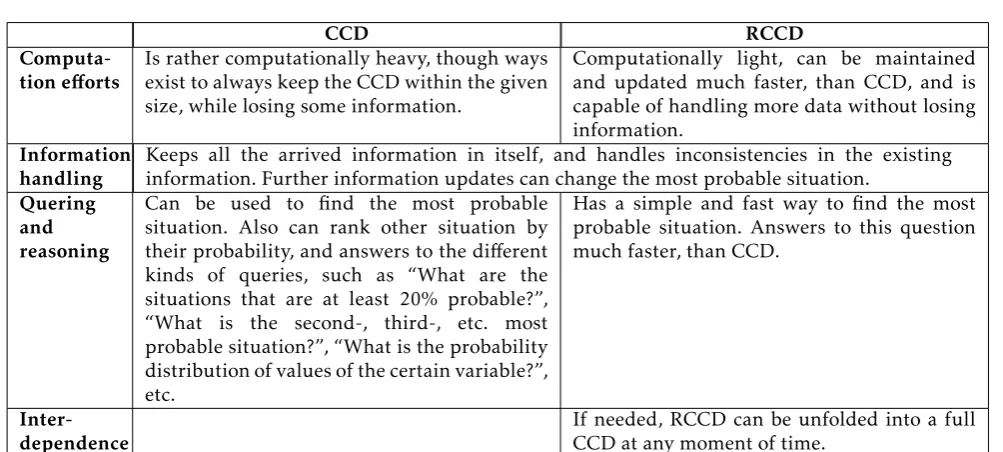
We introduced reduced context consistency diagrams (RCCD), novel data structures for reasoning about situ-ations with incomplete knowledge of the environment and context conflicts that cannot be unambiguously resolved. RCCD is able to find the most probable sit-uation at each moment of time, and can be unfolded into CCD to obtain the full quering functionality of the latter diagram. Our experiments show that diagrams can be efficiently maintained and computed in real-time and provide a considerable improvement in situation interpretation by correcting erroneous sensor readings. In table 4 we collect all the previously given information to present a concise comparison between the two structures. That should help to decide, which of the structures is better suited for given projects.
Acknowledgements. We want to thank prof. dr. Marco Aiello for useful comments about this work. We also want to thank Tuan Anh Nguyen for his valuable knowledge and his efforts in helping us to organize sensor experiments.
The research is supported by the EU project GreenerBuild-ings, contract FP7-258888, and by the Dutch NWO Smart Energy Systems program, contract 647.000.004.
References
[1] ADVANTICSYS(2012) URLwww.advanticsys.com. [2] Agrawal, R.andSrikant, R.(1994) Fast algorithms for
mining association rules.Proc 20th Int Conf Very Large
Data Bases VLDB1215: 487–499.
[3] Agrawal, R., Imieliński, T. and Swami, A. (1993)
Mining association rules between sets of items in large
databases.SIGMOD Rec.22: 207–216.
[4] Bu, Y.,Chen, S.,Li, J.,Tao, X.andLu, J.(2006) Context
consistency management using ontology based model.
Lecture Notes in Computer Science4254, 741–755. [5] Bu, Y.,Gu, T.,Tao, X.,Li, J.,Chen, S.andLu, J.(2006)
Managing quality of context in pervasive computing. In
QSIC ’06: Proc. Int. Conf. on Quality Software: 193–200. [6] Degeler, V. and Lazovik, A. (2011) Interpretation of
inconsistencies via context consistency diagrams. In
9th Annual IEEE International Conference on Pervasive Computing and Communications (PerCom’11): 20–27. [7] Han, J.,Cheng, H.,Xin, D.andYan, X.(2007) Frequent
pattern mining: current status and future directions.
Data Mining and Knowledge Discovery15: 55–86.
[8] Han, J., Pei, J. and Yin, Y. (2000) Mining frequent
patterns without candidate generation.SIGMOD Rec.29:
1–12.
[9] Henricksen, K. and Indulska, J. (2004) Modelling
and using imperfect context information. In Proc. of
the 2nd IEEE Annual Conf. on Perv. Computing and Communications: 33.
[10] Huang, Y., Ma, X., Tao, X., Cao, J. and Lu, J. (2008)
A probabilistic approach to consistency checking for pervasive context. InEUC ’08: Proc. IEEE/IFIP Int. Conf. on Embedded and Ubiquitous Computing: 387–393. [11] Huang, Y., Ma, X., Cao, J., Tao, X. and Lu, J.
(2009) Concurrent event detection for asynchronous
consistency checking of pervasive context. InIEEE Int.
Conf. Pervasive Computing and Communications: 1–9. [12] Jeffery, S.R.,Garofalakis, M.andFranklin, M.J.(2006)
Adaptive cleaning for RFID data streams. InProc. of the Int. Conf. on Very Large Data Bases: 163–174.
[13] Kaldeli, E., Warriach, E., Bresser, J., Lazovik, A.
andAiello, M.(2010) Interoperation, Composition and
Simulation of Services at Home. InICSOC,6470: 167–
181.
[14] Kong, H.,Xue, G.,He, X.andYao, S.(2009) A proposal
to handle inconsistent ontology with fuzzy owl. InProc. WRI World Congress on CS and Inf. Eng., 1: 599–603. [15] Lu, H., Chan, W. andTse, T. (2008) Testing pervasive
software in the presence of context inconsistency
resolution services. In Proc. Int. Conf. on Software
engineering: 61–70.
[16] Marcelloni, F.andAksit, M.(2001) Leaving
inconsis-tency using fuzzy logic. Information and Software
Tech-nology43(12): 725 – 741.
[17] Nguyen, T.A. and Aiello, M. (2012) Beyond indoor
presence monitoring with simple sensors. In Proc. 2nd
Int. Conf. on Pervasive and Embedded Computing and Communication Systems.
[18] Xu, C.andCheung, S.C.(2005) Inconsistency detection
and resolution for context-aware middleware support. In
Proc. Joint 10th European software engineering conference and 13th ACM SIGSOFT international symposium on Foundations of software engineering(ACM): 336–345. [19] Xu, C.,Cheung, S.C.andChan, W.K.(2006) Incremental
consistency checking for pervasive context. InICSE’06:
Proc. 28th Int. Conf. on Software Engineering: 292–301. [20] Xu, C., Cheung, S.C., Chan, W.K. and Ye, C. (2008)
[21] Xu, C., Cheung, S.C., Chan, W.K. and Ye, C. (2010)
Partial constraint checking for context consistency in
pervasive computing.ACM Trans. Softw. Eng. Methodol.
19(3): 1–61.
[22] Zaki, M.(2000) Scalable algorithms for association