© Global Society of Scientific Research and Researchers http://ijcjournal.org/
Combination of Multiple Acoustic Models with Multi-scale
Features for Myanmar Speech Recognition
Thandar Soe
a*, Su Su Maung
b, Nyein Nyein Oo
ca,b,cDepartment of Computer Engineering and Information Technology, Yangon Technological University,
11011Gyogone, Insein Township, Yangon, Myanmar
aEmail: [email protected]
bEmail: [email protected]
cEmail: [email protected]
Abstract
We proposed an approach to build a robust automatic speech recognizer using deep convolutional neural
networks (CNNs). Deep CNNs have achieved a great success in acoustic modelling for automatic speech
recognition due to its ability of reducing spectral variations and modelling spectral correlations in the input
features. In most of the acoustic modelling using CNN, a fixed windowed feature patch corresponding to a
target label (e.g., senone or phone) was used as input to the CNN. Considering different target labels may
correspond to different time scales, multiple acoustic models were trained with different acoustic feature scales.
Due to auxiliary information learned from different temporal scales could help in classification, multi-CNN
acoustic models were combined based on a Recognizer Output Voting Error Reduction (ROVER) algorithm for
final speech recognition experiments. The experiments were conducted on a Myanmar large vocabulary
continuous speech recognition (LVCSR) task. Our results showed that integration of temporal multi-scale
features in model training achieved a 4.32% relative word error rate (WER) reduction over the best individual
system on one temporal scale feature.
Keywords: acoustic modelling; deep convolutional neural networks; multi-scale features; Myanmar speech
recognition; ROVER combination.
---
1.Introduction
Automatic speech recognition (ASR) technique is widely used for transcribing audio speech to text. Due to the
strong power of modelling ability on temporal sequence, the hidden Markov model (HMM) has been intensively
used in ASR systems. With Gaussian mixture model (GMM) [13, 14] for feature statistic distribution estimation,
the GMM-HMM framework has dominated the ASR field for several decades. In a hybrid HMM with deep
neural network (DNN-HMM) framework, DNNs have been proposed to replace GMMs to compute state
observation probabilities for all tied states in HMM and have achieved a large gain in many challenging ASR
tasks [6, 7, 8, 17, 21]. Compared to GMM-HMM, the hybrid DNN-HMM can easily capture highly correlated
feature inputs under several consecutive speech frames within a relatively large context window, where GMM
can handle only one frame each time. Recently, convolutional neural networks (CNNs) have been attracting
much attention for acoustic models [18, 23, 24] because CNNs are able to explore local invariant and
hierarchical features in acoustic speech that DNNs cannot explore.
CNN attempts to capture structural locality in the feature space by applying convolutional filters. The extracted
feature is supposed to improve the classification performance. As we know, the target labels (e.g., senones or
phones) may have different temporal durations, i.e., the label category exists in different temporal scales. For
example, for stop phones the duration may be less than 30 milliseconds while for vowels the duration may be
more than 300 milliseconds. However, in most acoustic modelling using CNN, a fixed windowed input feature
of several frames corresponding to a target label is used in model training. If different temporal scale of input
feature is used for different target label training, the performance for ASR is supposed to be improved. In this
work, we focus on whether combination of temporal multi-scale features in model training can improve the
performance or not.
Combining information at multi-scales (either temporal or spatial) recently obtained great success in traffic sign
recognition [20], semantic segmentation [11] and depth map prediction [3]. To deal with the numerous
variations in acoustic space, it is possible to combine multiple acoustic models trained either with different
acoustic features or different model architectures using ensemble model combination techniques [1, 2, 10, 26].
All these techniques can leverage all structural information potentially available and increase the robustness of
the overall system. In this study, we introduced and evaluated a Myanmar ASR system with effective integration
of temporal multi-scale features. For a feature type from one temporal scale, a deep CNN acoustic model was
built. Models with different feature scales were combined in a Recognizer Output Voting Error Reduction
(ROVER) process on the N-best hypothesis lists during speech recognition.
Since 2015, we have built the first Myanmar LVCSR system [9] based on DNN-HMM acoustic model
framework. And later, a CNN-HMM baseline system has been built on the same task. The integration of
temporal multi-scale features in acoustic modelling is based on our CNN-HMM baseline. In the next section, we
discuss the basic structure and concepts of convolutional neural network. Section 3 introduces the basic
architecture of our system and describes the detailed components in our proposed model. Experiments and
2.Convolutional neural network
In speech recognition, deep convolutional neural networks consist of one or more convolutional layers followed
by pooling process, then on top of these CNN layers, one or several fully connected layers are stacked for
further feature processing and a softmax layer is stacked at last to output a normalized probability for acoustic
classification. Compared with DNNs, deep CNN restricts the network architecture with local connections and
weight sharing in the input layer so that it can explore local correlations in feature processing.
A convolutional layer does the convolutions on feature maps of the previous layer using filters, and then adds a
bias scalar to the corresponding feature map, followed by a non-linear operation [25]. Feature maps are the basic
units of convolutional and pooling layers.
In the typical speech inputs, the size of feature map can be represented as #times × #feadim, where #times is the
context window size of the input features and #feadim is the dimension of features (e.g., 38 dimensions
Mel-frequency cepstral coefficient (MFCC) is used in this work). Therefore, one way to extract multi-scale features
is to feed multiple input sizes by varying the context window sizes. Another way to extract multi-scale features
is by using filters with different sizes because filters in convolutional layers can be used as feature extractor to
capture time-frequency spectral variations.
The purpose of convolution is to extract features from input feature map using filter, where both the feature map
and the filter can be represented as matrices.
During convolution operation, the filter moves along the two dimensions of input feature and computes the dot
product to output a new feature map as:
h(ℓ)= σ (W(ℓ) * h(ℓ -1) + b(ℓ) ) (1)
Equation (1) shows the simplest situation where only one feature map exists in the previous layer, where h(ℓ -1)
and h(ℓ) are feature maps in two consecutive layers. The convolution operation (denoted as *) is performed
within the filter W(ℓ) and the feature map h(ℓ-1).
The bias b(ℓ) is added and finally the activation function σ(.), typically sigmoid or ReLU will be applied to
generate the outputs of the convolutional layer. When multiple feature maps are presented in the previous layer,
the results of convolution operations are accumulated first before adding the bias. The pooling layer performs
down-sampling on the feature maps of the previous layer and generates new ones with a reduced resolution. In
this work, max-pooling was used in all CNN layers. The max pooling operation involves picking up the
maximum from adjacent filter outputs. The extracted features are finally processed by fully connected layers.
3.Temporal multi-scale deep CNN acoustic models and combination
The basic architecture used in this work is illustrated in Fig. 1. There are two main parts: building multiple deep
different feature scales.
The outputs of all ASRs which provide complementary information sources for speech recognition are then
combined in a ROVER process on the N-best hypothesis lists to improve the performance of the whole system.
DCNN_1
DCNN_2
DCNN_N
Combination Recognition results Temporal multi-scale input
Figure 1: Design of the proposed temporal multi-scale features based deep CNN speech recognition system
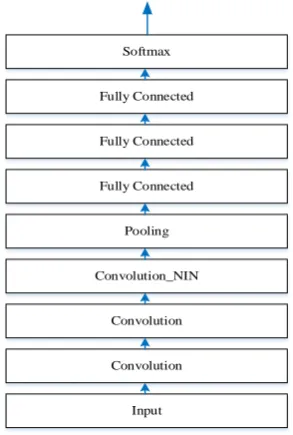
3.1.Acoustic model architecture
The proposed system is a combination of several deep CNNs acoustic models that share the same base
architecture and are trained on the same data in the same training procedure, but differ in their input feature
scales and filter sizes of the first convolutional layer. The base architecture of deep CNN is designed as shown
in Fig. 2. Our base architecture consisted three convolutional layers, followed by one pooling layer, three fully
connected layers and a softmax output layer. The third convolutional layer took the form of Network in Network
(NIN) structure [16].
Softmax
Fully Connected
Fully Connected
Fully Connected
Pooling
Convolution_NIN
Convolution
Convolution
Input
3.2.Decoding with language model
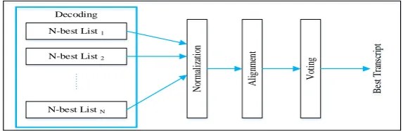
As shown in Fig. 1, the combination module is a ROVER process on the N-best hypothesis lists from the
decoding process of all models corresponding to different temporal scales. The decoding process for each model
is shown in Fig. 3. Decoding is the process to calculate which sequence of words is most likely to match to the
acoustic signal represented by the feature vectors. Initially, features were extracted from the recorded speech
signal as MFCCs. Decoding was then performed with an acoustic model, a pronunciation lexicon and a
language model. The lexicon is a list of words together with their corresponding phone sequence. Language
model (LM) is a fundamental component in ASR system. To perform optimally, a LM should be trained from
the same domain as the content that it will be applied to. The speech decoding is done with a weighted finite
state transducer (WFST)-based decoder. In this work, NICT SprinTra decoder [19] was used for decoding. For
each ASR, N-best hypothesis lists were extracted from the n-gram LM based lattices.
Language Model Pronunciation Lexicon DCNN Acoustic Model Decoder N-best hypothesis
Figure 3: Decoding to generate N-best hypothesis for temporal scale based ASR system
3.3.Combination of outputs from different acoustic models
Combining outputs from ASR systems with different acoustic models helps to provide auxiliary information for
improving speech recognition accuracy. ROVER was applied on the N-best lists generated from all ASRs. The
system combination procedure of the used ROVER approach is described in Fig. 4. After the N-best hypotheses
were obtained, the normalization was applied to scale the scores on the weighted best lists. After that, the
N-best lists from each ASR were aligned into a single confusion network, as in [12]. Once the network was
generated, a path with the lowest expected word error rate was extracted from all the N-best hypotheses with a
voting search process. Additionally, the word posterior probability was calculated as the word confidence by
summing the normalized scores for all N-best lists that contained the voted word.
N-best List 1
N-best List 2
N-best List N
4.Experiments
The experiments were carried out on 452 hours of conversational speech, of which 438.5 hours were used as the
training set and 13.5 hours were reserved as the validation set. The lexicon contains pronunciations for all words
and word fragments in the training data. The n-gram language model (LM) was built using the modified
Kneser-Ney smoothing method [22] with all training transcripts. The language model used in this task incorporates
236,171 words, as in lexicon. Evaluation was carried out on a 9.8 hours test dataset.
4.1.Feature extraction
Speech is recorded with a microphone with a sampling frequency of 16-kHz. Speech feature vectors are
represented as the MFCC, which is popularly used in traditional GMM-HMM based framework for ASR.
MFCC features were extracted using a 25-millisecond hamming window with 10 milliseconds frame rate. The
input features consisted of MFCCs (12 cepstral coefficients without energy) along with their first and second
order derivatives, in total 38 (12×3=36 with another two dimensions of the first and second order derivations of
log power energy).
4.2.Multi-scale deep CNNs acoustic models
Before training deep CNN-based (ASR1-ASR8) acoustic models, a basic context dependent triphone HMM
model with GMM based output probability was first trained to generate the senone alignments for later CNNs
training. Following triphone training of the GMMs, model-space discriminative training was done using the
boosted maximum mutual information (BMMI) criterion [5]. All models evaluated in this study used 3841
tied-triphone states (senones), determined by context dependent GMM-HMM system. The baseline GMM-HMM
model was built with Kaldi toolkit [4].
Based on the alignment from GMM-HMM model, the deep CNN based acoustic models were trained. The
architecture of deep CNNs used in this work consisted of three convolutional layers, followed by one pooling
layer, three fully connected layers and a softmax output layer. The input features used for all CNNs were 38
dimensions MFCC normalized with zero mean per speaker. The input layers were designed to process input
features with temporal context windows of 3, 9, 11, 13, 19, 23, 27 and 31 frames, therefore, the input layers
were with 114, 342, 418, 494, 722, 874, 1026 and 1178 dimensions for eight CNN acoustic models (denoted as
ASR1 to ASR8), respectively. The first convolutional layer had 180 filters with filter sizes (3×6) for ASR1, (9×6) for ASR2, (11×6) for ASR3, (13×6) for ASR4, (19×6) for ASR5, (23×6) for ASR6, (27×6) for ASR7 and (31×6) for ASR8, i.e., the receptive fields are with multi-temporal scales for the CNN. For all ASRs, the second and
third CNN layers had 180 filters with filter size (1×6) and (1×1), respectively. The stride size was fixed to 1. A max-pooling process with pooling size of (1×2) was used in this work. All three fully connected layers had 1024 nodes in each which were used to further transform the features extracted from CNNs. Sigmoid function was
used as the nonlinear activation function for hidden units. The softmax layer had 3841 output targets
corresponding to the HMM tied states (senones) in GMM-HMM ASR framework.
criterion, then a sequential discriminative training based on state level minimum Bayesian risk (sMBR) criterion
was adopted to further improve the model [15]. In the training, the standard back-propagation algorithm with
stochastic gradient descent based optimization was applied.
4.3.Evaluation criterion
The most common measure to evaluate the performance of a speech recognition system is word error rate
(WER). The hypothesized transcript is aligned to the reference transcript on words through the method of
dynamic programming. Three sets of errors are computed: substitution error (S) where a word is substituted by
ASR to a different word, insertion error (I) where a word presents in the hypothesis but absents in the reference,
deletion error (D) where a word presents in the reference but missing from the hypothesis. The accuracy (Acc) is
defined as:
T - D - S - I
Acc = 100%
T × (2)
where T is the number of words in the correct transcription, D is the number of deleted words, S is the number
of substituted words and I is the number of insertions. The error rate is closely related to the accuracy and
calculated as:
D + S + I
WER= 100% = 100% - Acc
T × (3)
4.4.Experimental results and discussion
We experimented with eight different models that differ mainly in the context window sizes and the filter sizes
of the first convolutional layer. Out of the eight models built, only models given better performance in the final
system combination are shown here.
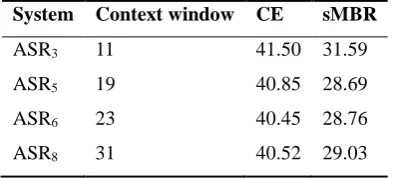
Table 1: Results (WER%) of ASRs on the test set using CE and sMBR criteria
System Context window CE sMBR
ASR3 11 41.50 31.59
ASR5 19 40.85 28.69
ASR6 23 40.45 28.76
ASR8 31 40.52 29.03
Table 1 compares the performance of our individual models using CE criterion and sMBR criterion. These
results illustrated that training with sMBR criterion produced lower word error rate by roughly 10% over
find that even the same utterance got different word error rates under different feature scales, as in Fig. 5.
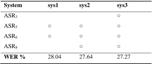
Table 2: Results (WER%) of different system combinations
System sys1 sys2 sys3
ASR3 ○
ASR5 ○ ○ ○
ASR6 ○ ○ ○
ASR8 ○ ○
WER % 28.04 27.64 27.27
To show the effectiveness of combining ASRs, different combinations of ASRs after the ROVER process is
listed in Table 2. From this table, we see that the combination of ASR6 and ASR5 , the system (sys1) achieved
28.04%.Through a series of experiments, performance constantly improved from 28.04% to 27.27% in sys3.
Therefore, the best ROVER combination was achieved 4.32% relative (1.42% absolute) word error rates
reduction over the individual system on one temporal scale feature.
Figure 5: Output transcripts of ASR6, ASR5 and ROVER over the same input utterance
Results in Fig. 5 demonstrate that the ROVER based combination clearly improve the decoding performance,
even with just two multi-scale deep CNNs in the model combination. Given the same speech to recognize, ASR6
and ASR5 output very similar results but with errors such as insertion (I) and substitution (S) of incorrect words.
Since the two ASRs are based on different feature scales, error segments across ASRs are uncorrelated.
Therefore, it is possible to improve the speech recognition accuracy by combining ASRs. Ultimately, we can
conclude from this experiment that each model has complementary information to achieving better performance.
5.Conclusions
In our study, we focus on using the complementary information from different deep CNNs acoustic models,
which differ mainly in context window sizes and filter sizes, to Myanmar speech recognition. We have shown
combination and ROVER based combination was efficient for improving recognition accuracy. We achieved a
4.32 % relative word error rates reduction with the N-best list based ROVER process. For future research, we
expect additional gains from using attention model which can learn to weight the multiple scales according to
the input feature scales.
6.Recommendations
This work describes an approach to build a robust automatic speech recognizer that can be utilized for
transcription of Myanmar audio speech to text.
Acknowledgments
This work was done during the first author’s internship period in National Institute of Information and
Communications Technology (NICT), Kyoto, Japan. We are grateful for support from NICT.
References
[1] B. Hoffmeister, C. Plahl, P. Fritz, G. Heigold, J. Loof, R. Schluter, et al. “Development of the 2007
RWTH mandarin LVCSR system,” In Proc. of IEEE 2007 Workshop on Automatic Speech
Recognition and Understanding (ASRU), 2007.
[2] C. Breslin and M.J. Gales. “Generating complementary systems for speech recognition,” In Proc.
INTERSPEECH, 2006.
[3] D. Eigen, C. Puhrsch and R. Fergus. “Depth map prediction from a single image using a multi-scale
deep network,” In Proc. NIPS, 2014, pp. 2366–2374.
[4] D. Povey, A. Ghoshal, G. Boulianne, L. Burget, O. Glembek and N. Goel. “The kaldi speech
recognition toolkit,” In Proc. of IEEE 2011 Workshop on ASRU, 2011.
[5] D. Povey, D. Kanevsky, B. Kingsbury, B. Ramabhadran, G. Saon and K. Visweswariah. “Boosted
MMI for model and feature-space discriminative training,” In Proc. International Conference on
Acoustics, Speech and Signal Processing (ICASSP), 2008.
[6] G.E. Dahl, D. Yu, L. Deng and A. Acero. “Context-dependent pre-trained deep neural networks for
large-vocabulary speech recognition.” IEEE Transactions on Audio, Speech, and Language Processing,
vol. 20, no. 1, pp. 30-42, 2012.
[7] G. Heigold, V. Vanhoucke, A. Senior, P. Nguyen, M. Ranzato, M. Devin, et al. “Multilingual acoustic
models using distributed deep neural networks,” In Proc. of ICASSP, 2013, pp. 8619–8623.
[8] G. Hinton, L. Deng, D. Yu, G.E. Dahl, A. Mohamed, N. Jaitly, et al. “Deep neural networks for
acoustic modeling in seech recognition: The shared views of four research groups.” Signal Processing
Magazine, IEEE, vol. 29, no. 6, pp. 82-97, 2012.
[9] H.M.S. Naing, A.M. Hlaing, W.P. Pa, X. Hu, Y.K. Thu, C. Hori, et al. “A Myanmar large vocabulary
continuous speech recognition system,” In Proc. of APSIPA Annual Summit and Conference, 2015, pp.
320-327.
[11]J. Long, E. Shelhamer and T. Darrell. “Fully convolutional networks for semantic segmentation,” In
Proc. CVPR, 2015.
[12]L. Mangu, E. Brill and A. Stolcke. “Finding consensus among words: lattice-based word error
minimization,” In Proc. Eurospeech, 1999, pp. 495-498.
[13]L.R. Rabiner. “A tutorial on hidden Markov models and selected applications in speech recognition.”
In Proc. IEEE, vol.77, no. 2, Feb. 1989.
[14]L.R. Rabiner and B.H. Juang. Fundamentals of Speech Recognition, Prentice-Hall, Englewood Cliff,
New Jersey, 1993.
[15]M. Gibson and T. Hain. “Hypothesis spaces for minimum Bayes risk training in large vocabulary
speech recognition,” In Proc. INTERSPEECH, 2006, pp. 2406-2409.
[16]M. Lin, Q. Chen and S. Yan. “Network in network,” arXiv preprint arXiv: 1312.4400, 2013.
[17]N. Kanda, R. Takeda and Y. Obuchi. “Elastic spectral distortion for low resource speech recognition
with deep neural networks,” In Proc. of ASRU, 2013, pp. 309–314.
[18]O. Abdel-Hamid, A. Mohamed, H. Jiang, L. Deng, G. Penn and D. Yu. “Convolutional neural
networks for speech recognition.” IEEE/ACM Transactions on Audio, Speech and Language
Processing, vol. 22, no. 10, pp. 1533-1545, 2014.
[19]P.R. Dixon, C. Hori and H. Kashioka. “Development of the SprinTra WFST speech decoder,” NICT
Res. J. 59 (3/4), pp.15-20, 2012.
[20]P. Sermanet and Y. LeCun. “Traffic sign recognition with multi-scale convolutional networks,” In
Proc. of IEEE 2011 International Joint Conference in Neural Networks (IJCNN), 2011, pp. 2809–2813.
[21]P. Shen, X. Lu, N. Kanda, M. Saiko and C. Hori. “The NICT ASR system for IWSLT 2014,” In Proc.
IWSLT, 2014, pp. 113–118.
[22]S.F. Chen and J. Goodman. An Empirical Study of Smoothing Techniques for Language Modeling,
TR-10-98, Computer Science Group, Harvard University, 2008.
[23] T.N. Sainath, A. Mohamed, B. Kingsbury and B. Ramabhadran. “Deep convolutional neural networks
for LVCSR,” In Proc. ICASSP, 2013, pp. 8614-8618.
[24]T. Sercu, C. Puhrsch, B. Kingsbury and Y. LeCun, “Very deep multilingual convolutional neural
networks for LVCSR,” In Proc. ICASSP, 2016, pp. 4955-4959.
[25]Ujjwalkarn. (2016). “An explanation of CNN.” [On-line], Available:
https://ujjwalkarn.me/2016/08/11/intuitive-explanation-convnets/ [Aug. 22, 2017].
[26]X. Cui, J. Xue, B. Xing and B. Zhou. “A study of bootstrapping with multiple acoustic features for