Constructing Small-Bias Sets from Algebraic-Geometric Codes

www.theoryofcomputing.org

Constructing Small-Bias Sets from

Algebraic-Geometric Codes

∗

Avraham Ben-Aroya

Amnon Ta-Shma

Received February 21, 2011; Revised October 29, 2012; Published February 20, 2013

Abstract: We give an explicit construction of anε-biased set overkbits of size

O

k

ε2log(1/ε)

5/4

.

This improves upon previous explicit constructions whenε is roughly (ignoring logarith-mic factors) in the range[k−1.5,k−0.5]. The construction builds on an algebraic-geometric code. However, unlike previous constructions, we use low-degree divisors whose degree is significantly smaller than the genus.

ACM Classification:F.2.2, G.2

AMS Classification:94B27, 12Y05

Key words and phrases:small-bias sets, algebraic geometry, AG codes, Goppa codes

1

Introduction

Explicitly constructing combinatorial objects with certain properties (such as expander graphs, extractors, error correcting codes and others) is an intriguing challenge in computer science. Often, it is easy to verify that a random object satisfies the required property with high probability, while it is difficult to pin down such an explicit object.

∗_{A preliminary version of this paper appeared in FOCS 2009 [3].}

†_{Supported by the Adams Fellowship Program of the Israel Academy of Sciences and Humanities, and by the European}

Commission under the Integrated Project QAP funded by the IST directorate as Contract Number 015848.

In most cases it is believed (and sometimes proven) that a random object is nearly optimal. Therefore, giving an optimal explicit construction becomes a derandomization problem. There are, however, rare cases in which explicit constructions outperform naive random constructions. Perhaps the most remarkable example of this type is that of algebraic-geometric codes (AG codes). In the seminal work of Tsfasman et al. [10] it was shown that there are algebraic-geometric codes over constant size alphabets that lie above the Gilbert-Varshamov bound, a bound that random codes achieve and that was believed to be optimal at the time.

The important case ofbinaryerror correcting codes is still open. In the binary case, the Gilbert-Varshamov bound gives the best known (explicit or non-explicit) codes to date. For codes with distance close to half, the bound shows that random linear codes of lengthn=O(k/ε2)are [n,k,(1/2−ε)n]2 codes. Finding an explicit construction that attains this bound is an open problem.

Another closely related question is that of finding an[n,k,(1/2−ε)n]2binary code, in which the relative weight of every non-zero codeword is in the range[1/2−ε,1/2+ε]. Such codes are called ε-balancedand they are related to another kind of combinatorial objects calledε-biased sets. Anε-biased set is a setS⊆ {0,1}k such that for every non-empty subsetT ⊆[k], the binary random variableL

i∈Tsi, wheresis sampled uniformly fromS, has bias at mostε. It turns out thatε-biased sets are justε-balanced codes in a different guise: the rows of a matrix whose columns generate anε-balanced code form an ε-biased set, and vice versa. In terms of parameters, an[n,k]2ε-balanced code is equivalent to anε-biased setS⊆ {0,1}k of sizen.

The status of ε-balanced codes is similar to that of [n,k,(1/2−ε)n]2 codes. In both cases the probabilistic method gives non-explicit[n,k]2ε-balanced codes withn=O(k/ε2), whereas the best lower bound is

n=Ω k

ε2log(1_ε)

!

.

For a discussion of these bounds see [2, Section 7].

There are several explicit constructions of such codes. Naor and Naor [7] give a construction withn=k·poly(ε−1), which was later improved in [1] ton=O(k/ε3). Alon et al. [2] establish the incomparable bound

n=O k

2

ε2log2(k_ε)

!

.

Concatenating algebraic-geometric codes with the Hadamard code gives

n=O k

ε3log(1_ε)

!

.

In this paper we show an explicit construction of an[n,k]2ε-balanced code with

n=O k

ε2log(1_ε)

!5/4

,

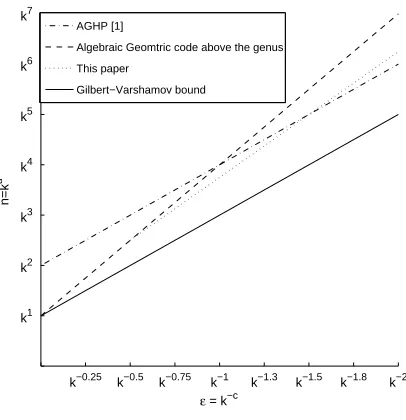
ε = k−c

n=k

d

k−0.25 k−0.5 k−0.75 k−1 k−1.3 k−1.5 k−1.8 k−2 k1

k2 k3 k4 k5 k6 k7

AGHP [1]

Algebraic Geomtric code above the genus This paper

Gilbert−Varshamov bound

Figure 1: Constructions ofε-biased sets forε=k−c.

The construction is simple and can be described by elementary means. We first take a finite fieldFq of the appropriate size. We then carefully choose a subsetAofFq×Fq. The elements in theε-biased set are indexed by pairs((a,b),c)∈A×_Fq. For each((a,b),c)∈A×Fqthe corresponding element is the bit vector h(ai_bj_),ci

2

i,j, where(i,j)range over all integersi,jwhose sum is bounded by an appropriately chosen parameter and the inner product is of the binary representation of the elements inFq. The analysis of the construction relies on Bézout’s Theorem.

To put the construction in context, we need to move to the terminology of algebraic function fields. AG codes areevaluationcodes where a certain set ofevaluation functionsis evaluated at a chosen set of

The codeC(G)has the following parameters.

• Thelengthof the code is the number of evaluation points and is denoted byN=N(F).

• Thedistanceof the code isN−deg(G), where deg(G) is the degree ofG(formally defined in

Section 3).

• Thedimensionof the code, dim(G), is the dimension of the vector space of evaluation functions.

When the “degree” ofGis larger than thegenus gof the function fieldF(again, defined inSection 3) the Riemann-Roch Theorem [8, Thm I.5.17] tells us exactly what the dimension dim(G)is, and it turns out that

dim(G) =deg(G)−g+1.

This almost matches the Singleton bound, dim(G)≤deg(G) +1, except for a loss ofg. Thus, our goal is to get as many evaluation points as possible while keeping the genus small. Indeed, a lot of research has been done on the best possible ratio between the length of the codeN(F)and the genusg. The bottom line of this research, roughly speaking, is thatN(F)can be larger than the genus by at most a multiplicative√q−1 factor and this is essentially optimal.

A simple check shows that when deg(G)is larger than the genus, an AG code concatenated with the Hadamard code cannot giveε-balanced codes withnbetter than

O k

ε3log(1_ε)

!

(seeSection 3.2). In contrast, our construction takes as an outer code an AG codeC(G)where deg(G)is much smaller than the genus, and we show that this leads to a better code.

A natural question is whether theε-balanced codes we achieve are the best binary codes one can achieve using this approach. We do not know the answer to this question. When deg(G)is smaller than the genus, one cannot use the Riemann-Roch Theorem, and estimating dim(G)is often a challenging task. Furthermore, dim(G)now depends onGitself, and not just on its degree as before. However, we can formulate the question as follows. The important thing for us is not the best possible ratio between the number of evaluation pointsN(F)and the genus. Instead, we are interested in the best possible ratio betweenN(F)and deg(G), whereGis alow-degreedivisor having alarge dimension.

Following the preliminary version of our work [3], Felipe Voloch [11] used a variant of Castelnuovo’s bound to show our approach cannot lead to error correcting codes approaching the Gilbert-Varshamov bound. We show that a careful analysis of Voloch’s argument implies that allk-dimensionalε-balanced codes built using our approach must have length

n=Ω k

ε2.5log2(1_ε)

!

.

2

A self-contained elementary description of the construction

We first recall the definition of anε-biased set.

Definition 2.1. A setS⊆ {0,1}k isε-biasedif for every nonemptyT ⊆[k],

1

|S|

∑

s∈S

(−1)∑i∈Tsi

≤ε.

The construction Givenkandε, letp=2`be a power of 2 in the range

" 1 2 k ε2

1/4

,

k

ε2

1/4#

.

That is,

1 16

k

ε2 ≤p

4_≤ k

ε2.

Defineq=p2andr=εp3. LetFqdenote the finite field with qelements andFp its subfield with p elements. Consider the vector space of bivariate polynomials overFqwith total degree at mostr/(p+1).

V =

φ∈Fq[x,y] : deg(φ)≤ r p+1

= Span

xiyj : i+j≤ r

p+1

.

We denote the dimension of this space (overFq) byk0. It follows that

k0=Θ

r2 p2 =Θ

ε2p6

p2

=Θ ε2p4=Θ(k).

LetA⊆_Fq×Fqbe the set of roots of the polynomialyp+y−xp+1. Theε-biased set overk0bits that we construct is

S=

bin(aibj),bin(c)_2i+j≤ r p+1

: (a,b)∈Aandc∈Fq

,

where bin :Fq→Z22`is any isomorphism between the additive group ofFqand the vector spaceZ22`and

h·,·i2denotes inner product overZ22`.

The analysis Clearly,|S|=q|A|. We further claim:

Claim 2.2. The cardinality of A is p3.

Proof. The trace function Tr(y) =yp+ymapsFqtoFp. We claim that for everyα ∈Fp, the number of solutions inFqto Tr(y) =α is p. To see this, observe that Tr is a linear function. Hence, the set of solutions to Tr(y) =0 is a subgroup ofFqthat has at most pelements. For everyα∈Fp, the set of solutions to Tr(y) =α is either empty or a coset of this subgroup. As every element ofFqis in one of these cosets, it must be the case that for everyα∈Fpthere are exactlypsolutions.

The norm functionN(x) =xp+1also mapsFqtoFp. Thus, for everyα∈Fqthere are exactlypvalues

In order to bound the biasε, we need to invoke Bézout’s theorem, reviewed below. First, we need to show that the bivariate polynomialyp+y−xp+1is irreducible. We do this using Eisenstein’s Criterion:

Theorem 2.3(Eisenstein’s Criterion [6, Thm 3.1]). Let U be a unique factorization ring and let K be its field of fractions. Let f(x) =∑ni=0aixi be a polynomial of degree n≥1in U[x]. Letρ be a prime of U , and assume:

• an6=0 (mod ρ),

• for every i<n, ai=0 (modρ),

• a06=0 (mod ρ2).

Then f(x)is irreducible in K[x].

With that we conclude:

Claim 2.4. The polynomial yp+y−xp+1is irreducible overFq.

Proof. This follows from Eisenstein’s Criterion. The unique factorization ring we consider isU=Fq[y]. The prime element we use isρ=y. The leading coefficient isap+1=−1 and−16=0 (mod y). Every other coefficient except the last is 0, hence it is 0 (mod y). The last coefficient isa₀=yp+y=0 (mod y). Finally, sincep≥2,yp=0 (mod y2)buty6=0 (mod y2), hencea0=yp+y6=0 (mody2). Therefore the univariate polynomial (inx) is irreducible over the field of fractions. As one of the coefficients is−1, it follows that the bivariate polynomial is irreducible over the fieldFq(see [6, Thm 2.3]).

We are now ready to recall Bézout’s Theorem and apply it to proveSis indeedε-biased.

Theorem 2.5(Bézout’s Theorem [4, Section 5.3]). Supposeφ andψare two bivariate polynomials over

some field. Ifφandψhave more thandeg(φ)·deg(ψ)common roots then they have a common factor.

Theorem 2.6. For every k andε such thatε<1/

√

k, S is anε-biased set over k0=Ω(k)bits of size

O

k

ε2

5/4

.

Proof. ByClaim 2.2,

|S|=|A| ·q=p5=O

k

ε2

5/4

.

We now show thatSisε-biased. LetT ⊆[k0]be some non-empty set. We identify[k0]with the set

(i,j) : i+j≤ r

p+1

Lets∈Sbe an element specified by the pair((a,b),c)∈A×_Fq. Then,

∑

s₍i,j)=

∑

bin(aibj),bin(c)₂= *

bin

_∑

(i,j)∈T aibj

!

,bin(c) +

2

.

The polynomialφT=∑(i,j)∈Txiyj is a non-zero polynomial. Clearly, for any(a,b)which is not a root ofφT, the inner product will be unbiased when ranging overc(i. e., exactly half of the values forc will make the inner product 0). From the assumptionε<1/

√

kit follows that deg(φT)<p+1, since

deg(φT) p+1 ≤

r

(p+1)2 <εp≤k 1/4√

ε<1.

Hence, byClaim 2.4it follows thatφT andyp+y−xp+1have no common factors. Therefore, by Bézout’s theorem we conclude that the number of roots ofφT that are inAis at most(_p+r₁)·(p+1) =rand

1

|S|

∑

s∈S

(−1)∑i∈Tsi

≤ r

|A|=ε.

Remark 2.7. The above construction can be improved to anε-biased set of size

O k

ε2log(1_ε)

!5/4

for everykandε such that q ε

log(1_ε)

<√1

k.

To achieve this we choose

p=Θ k

ε2log(1_ε)

!1/4

.

We then observe that instead of taking a basis forV overFq, we can actually afford to take a basis overF2. Finally, we need to use the fact that by the constraints we have onε, it follows that log(1/ε) =Θ(log(p)). When we restate the construction in the terminology of algebraic function fields, we also include this improvement.

3

Restating the construction in the terminology of algebraic function fields

Without putting the above construction in the proper context, it may appear coincidental. We now describe the general framework of algebraic-geometric codes and explain why the above construction fits into this framework.

3.1 Algebraic geometry

LetFqdenote the finite field withqelements. The polynomial ringFq[x], wherexis transcendental overFq, is the set of allpolynomialsinxwith coefficients inFq. Therationalfunction fieldFq(x), where xis transcendental overFq, contains allrationalfunctions inxwith coefficients inFq. A fieldFis an algebraic function field overFq, denotedF/Fq, ifF is afinitealgebraic extension ofFq(x).

Aplace PofF/Fqis a maximal ideal of some valuation ringOof the function field. We denote byOPthe valuation ring that corresponds to the placeP. We denote byvP thediscrete valuationthat corresponds to the valuation ringOP. Therefore, we can writePandOPas

P={y∈F : vP(y)>0} and OP={y∈F : vP(y)≥0}.

SincePis a maximal ideal,FP=OP/Pis a field. In fact, it is a finite field [8, Proposition I.1.14]. For everyy∈OP,y(P)denotesy (modP)and is an element ofFP. It can be thought of as the evaluation of the functionyat the “evaluation point”P. The degree of a placePis defined to be deg(P) = [FP:Fq], i. e., the dimension ofFP as a vector space overFq. In particular, if a placePis of degree 1 thenFPis isomorphic toFqand the evaluation ofyat the placePis an element ofFq.

We proceed with a simple example that illustrates the above notions.

Example 3.1. The rational function fieldFq(x)/Fqis the simplest algebraic function field. For every irreducible polynomialp(x)letOpdenote the set of rational functionsr(x) =u(x)/w(x)whose denom-inatorw(x)is not divisible byp. The setOpforms a ring. Furthermore, for every rational functionr, eitherrorr−1belongs toOp, makingOpa valuation ring. The placePpis the set of rational functions r(x) =u(x)/w(x)for whichpdividesubut does not dividew.

There is exactly one more valuation ring in Fq(x). Let O∞ denote the set of rational functions

r(x) =u(x)/w(x)for which deg(w)≥deg(u). Again,O∞is a ring and furthermore, for every rational

functionr(x) =u(x)/w(x), eitherrorr−1belongs toO_∞, makingO_∞a valuation ring. The placeP_∞is the set of rational functionsr(x) =u(x)/w(x)for which deg(w)>deg(u).

For an irreducible polynomialp, the discrete valuationvpcorresponding toOpis defined as follows. For a polynomialu(x)∈Fq[x],vp(u)is the largest integerksuch that pkdividesu. For a rational function r(x) =u(x)/w(x),vp(r) =vp(u)−vp(w). Thus,vp(r)counts the number of zeroes (or poles) thatrhas when the irreducible polynomialp(x)is zero. Ifpis linear, i. e.,p(x) =x−α,vp(r)counts the number of zeroes (or poles) the polynomialp(x)has when settingx=α. If in additionr=u/wbelongs toOp, i. e., pdoes not dividew, thenr(Px−α) =rmod(x−α)is well defined, and, in fact, is the elementu(α)/w(α)

inFq.

The discrete valuationv∞corresponding toO∞is defined as follows. For a polynomialu(x)∈Fq[x], v_∞(u)is−deg(u). For a rational functionr(x) =u(x)/w(x),v_∞(r) =v_∞(u)−v_∞(w) =deg(w)−deg(u). Thus,v∞(r)counts the number of zeroes (or poles) thatrhas whenx=∞. Ifr(x) =u(x)/w(x)belongs

toO∞, i. e., deg(w)≥deg(u), thenr(P∞)is well defined, and is either zero (if deg(w)>deg(u)) or the

elementuk/wkinFq, whereukandwkare the leading coefficients of the polynomialsuandwrespectively.

We letPF denote the set of places ofF, andN(F)the number of places ofdegree1 inF/Fq.N(F)is always finite.DF is the free abelian group over the places ofF. Adivisoris an element in this group, i. e., it is a formal sumG=∑P∈_PFnPPwithnP∈Zand wherenP6=0 for only a finite number of places. We

finite. We sayG1≥G2ifG1is component-wise larger thanG2, i. e.,vP(G1)≥vP(G2)for every placeP. Thesupportof a divisorGis Supp(G) ={P∈PF : vP(G)6=0}.

Each element 06=x∈F is associated with two divisors. The first is called theprincipal divisorofx

and it is defined by

(x) =

_∑

vP(x)P.

The degree of a principal devisor is always 0. The second is thepole divisorofxand it is defined by

(x)∞=

∑

P:vP(x)<0

−vP(x)P.

Ifx∈F\Fqthen deg((x)∞) = [F:Fq(x)].

Example 3.2(Continued fromExample 3.1). Letu∈_Fq[x]be an arbitrary nonconstant polynomial. Then, uhas a pole atP∞(sincev∞(u)<0) and zero atPp, for every irreducible polynomialpthat dividesu(since vp(u)>0). Thus,(u)∞=deg(u)P∞and deg((u)∞) =deg(u). Also, it turns out thatdeg(Pp) =deg(p). Thus,∑pvp(u)is the number of irreducible factorsuhas, and∑pvp(u)deg(Pp)is the degree ofu. In total, deg((u)) =0.

For a divisorG, we define theRiemann-Roch spaceL(G)to be:

L(G) ={x∈F : (x)≥ −G} ∪ {0}.

Example 3.3(Continued from Examples3.1and3.2). For the divisorG=kP∞the Riemann-Roch space

L(G)is the set of all polynomials of degree at mostkoverFq.

The setL(G)is a vector space and furthermore has finite dimension. We define the dimension ofG

by dim(G) =dimL(G)and we use the two notations interchangeably. The fact that the degree of each principal divisor is 0 implies that if deg(G)<0 then dim(L(G)) =0.

3.1.1 Geometric Goppa codes

A Goppa code is specified by a triplet(F,Y,G), whereF/Fqis a function field,Y ={P1, . . . ,Pn}is a set of places of degree 1 andGis an arbitrary divisor with no support over any place inY. Notice that for anyx∈L(G),vPi(x)≥0 and thereforex∈OPi andx(Pi)∈Fq. The triplet(F,Y,G)specifies the code:

C(Y;G) ={(x(P1), . . . ,x(Pn)) : x∈L(G)} ⊆Fqn.

Claim 3.4([8, Cor II.2.3]). Ifdeg(G)<n then C(Y;G)is an[n,dim(G),n−deg(G)]linear code over

Fq.

Theorem 3.5([8, Thm I.5.17]). Ifdeg(G)≥2g−1thendim(G) =deg(G)−g+1.

This, in particular, allows one to easily compute the dimension of the code when deg(G)≥2g−1. The only remaining question is whether there are function fieldsF/Fqwith a large numberN=N(F)of evaluation points (i. e., degree 1 places) and a small genusg. Anegativeanswer to that question is given by the Hasse-Weil bound:

Theorem 3.6(Hasse-Weil bound [8, Thm V.2.3]). Let F/Fqbe a function field of genus g. Then, the number N of places of degree one satisfies N≤(q+1) +2√qg.

The Drinfeld-Vl˘adu¸t bound tells us that whengtends to infinity, the bound can be strengthened by about a factor of 2, and roughly speaking,N≤g(√q−1). This is tight for prime power squaresq.

On the positive side, the good news is that following much research, there are several beautiful explicit constructions that meet the Drinfeld-Vl˘adu¸t bound, and we refer the interested reader to the beautiful survey paper [5, Chapter 1].

In this paper we look at divisorsGwhose degree is smaller than the genus. Much less is known about such small-degree divisors. In this regime, dim(G)depends on the divisorGitself, and not only on its degree, as is the case when deg(G)≥2g−1. For some special algebraic function fields the vector space L(G)(and therefore also its dimension) is known in full. We discuss this below.

3.2 Concatenating AG codes with Hadamard

In this section we consider the concatenation of an outer code with the Hadamard code. If the outer code is an[n1,k1,d]qcode andqis a power of two, then concatenating it with the[q,logq,q/2]2Hadamard code gives an[n=n1q,k=k1logq]2code that isε= (n1−d)/n1balanced, because non-zero symbols in the outer code expand by the concatenation to perfectly balanced blocks.1

Using a[q,k₁,q−k₁+1]qReed-Solomon code as the outer code, one gets an[n=q2,k=k1logq]2 code that isε<k1/qbalanced. Rearranging the parameters, this gives an[n,k]2ε-balanced code with

n=O k

εlog(k_ε) !2

. (3.1)

This is one of the constructions in [2].

Taking the outer code to be an[N,dim(G),N−deg(G)]qAG codeC(Y;G)overFqand concatenating it with Hadamard, we get an[n=Nq,k=dim(G)logq]2code that isε=deg(G)/N balanced. We can choose an AG code which uses a curve of genusgwithN=Θ(g√q)degree 1 places (the asymptotic is overggoing to infinity). Picking the divisorGto be of degree deg(G)≥2gand settingq=1/ε2results in

N=deg(G)

ε =

dim(G) +g−1

ε =Θ

k

εlog(1_ε)

!

,

1_{Ifqis a power of 2, then the resulting concatenated code is linear. Concatenation is well defined even whenqis not a power}

of 2. In such a case we embedFqintoF2dlogqeusing any one-to-one mapping. The resulting (non-linear) code has essentially

where the second equality follows from the Riemann-Roch Theorem. Thus, we get anε-balanced code of length

n=Nq=O k

ε3log(1_ε)

!

. (3.2)

In fact, if one takes an AG code overFqwith large genusg≥

√

qthen

N≥ dim(G)

ε =

k

εlogq and q=Ω

1

ε2

and equation (3.2) is tight. Taking an AG code with a small genusg≤√qis essentially equivalent to taking a Reed-Solomon outer code and cannot be better (up to constant factors) than equation (3.1). In what follows, we show one can improve on both bounds when the AG code has degree much smaller than the genus.

So we now turn our attention to the case where deg(G)≤2g−1. In this case dim(G)depends on the divisorGand not just its degree. One special case is the case whereG=rQ,r∈_NandQis a place of degree 1. For any suchr, dim(rQ)is either equal to dim((r−1)Q)or to dim((r−1)Q) +1. In the former caseris said to be agap numberofQ. The Weierstrass Gap Theorem [8, Thm I.6.7] says that for any placeQthere are exactlyg=genus(F/Fq)gap numbers, and they are all in the range[1,2g−1].

The non-gap numbers (also calledpole numbers) form a semigroup ofN(i. e., a set that is closed under addition). This semigroup is sometimes referred to as theWeierstrass semigroupofQ. We say that a semi-groupSisgenerated by a set of elements{gi}, if eachgi∈Sand, furthermore, every element s∈Scan be expressed ass=∑aigiwithai∈N.

The structure of the Weierstrass semigroup is crucial to our construction. We know that there are exactlygnon-gap elements of this semigroup in the range[1,2g]. If these elements are too concentrated on the upper side of the range then the behavior of dim(rQ)will be very similar to the case wherer>2g−1. Thus, our goal is to find a function fieldF that has many places of degree 1, say,N(F)≥Ω(g√q), while at the same timeF has a degree 1 placeQwith a “good” Weierstrass semigroup.

3.3 The construction

Letpbe a prime power andq=p2. The Hermitian function field overFq(see [8, Lemma VI.4.4]) can be represented as the extension fieldFq(x,y)of the rational function fieldFq(x)withyp+y=xp+1. This function field has 1+p3places of degree one. First, there is the common poleQ∞ofxandy. Moreover,

for each pair(α,β)∈Fq with βp+β =αp+1 there is a unique place Pα,β of degree one such that

x(P_α,β) =α andy(P_α,β) =β and we already saw there arep3such pairs. The genus of the Hermitian function field isg=p(p−1)/2.

For the outer code we take the Goppa codeCr=C(Y,G=rQ∞), whereY is the set of all degree 1

placesP_α,β mentioned above andr=εp

3_{. The Weierstrass semigroup ofGis generated bypandp+1,}

and a basis forL(G) =L(rQ∞)is

xiyj : j≤p−1 andip+j(p+1)≤r .

The dimension of the code is

We can now see the similarity between this construction and the one inSection 2. The parameterris chosen such that the constraintip+j(p+1)≤rforces j≤p−1. Therefore, both use evaluations of low degree bivariate polynomials over the same set ofp3points.2

Theorem 3.7. For every k and everyε such that

ε

p

log(1/ε)

≤√1

k,

there exists an explicit[n,Ω(k)]2code that isε-balanced, with

n=O

k

ε2log(1/ε)

5/4

.

Proof. For a givenkandε, let

p∈ " 1 2 k

ε2log(1/ε)

1/4

,

k

ε2log(1/ε)

1/4#

be a power of two. It can verified that

1

16p4 ≤ ε ≤ 1 p as 1 p ≥

ε2log(1/ε)

k

1/4

≥

ε2log(1/ε)· ε

2

log(1/ε)

1/4 = ε

and

ε = ε2·1 ε ≥ ε

2_·log

1

ε

≥ k

16p4 ≥ 1 16p4,

and so log(1/ε) =Θ(log(p)).

Letr=εp3and letFqbe the field withq=p2elements. LetF denote the Hermitian function field overFqand letY denote its set of places of degree 1, excludingQ∞. This implies that|Y|=p3. Define

the divisorGto beG=rQ∞. Sincer≤p2,

dim(rQ∞)≥

r

2(p+1) 2

=Ω ε2p4=Ω

k

log(p)

.

ByClaim 3.4, the Goppa code that is obtained from the triplet(F,Y,G)is a

p3,Ω

k

log(p)

,p3−r

p2

2_{The only slight difference is that in this construction we take all bivariate polynomials with boundedweightedtotal degree.}

code. Concatenating this code with Hadamard gives a[p5,Ω(k)]2code that isε-balanced (sincer/p3=ε). Now, by our choice ofp, it follows that

k

ε2log(_ε1) =Θ(p 4₎

and therefore

n=p5=O 

 k

ε2log(_ε1)

!5/4



as desired.

4

Limits of the approach

As explained inSection 3.1.1, the genus measures the maximal loss in dimension compared to the degree. The Drinfeld-Vl˘adu¸t bound implies that the number of evaluation points (which is bounded by the number of degree one placesN(F)) is at mostO(g√q) whenN(F)q. InSection 3.2we saw this implies that when deg(G)>2g, concatenating the best AG codeC(Y;G)with the Hadamard code cannot give ε-balanced codes of dimensionkand length

n=o

k

ε3log(1/ε)

.

Our construction shows that substantially better results are possible when deg(G)g. Namely, we show that there exists a codeC(Y;G)with deg(G)gsuch that when this code is concatenated with Hadamard, it gives ak-dimensionalε-balanced code of length

n=O

k

ε2log(1/ε)

5/4!

.

It is therefore natural to ask what are the limits of our approach. More concretely we ask what are the best codes one can construct by concatenating an AG code with a Hadamard code? Let us state the question precisely. We look at constructions of the following structure:

• An outer AG codeC=C(Y;G), defined by an algebraic function fieldF/Fq, a set of degree 1 placesY and a divisorG∈DF with no support over any place inY.

• An inner Hadamard code.

In the analysis we viewCas a[|Y|,dim(G),|Y| −deg(G)]qcode, and then the concatenated code has parameters

|Y|q,dim(G)log(q), 1

2−

deg(G)

|Y|

2

.

Notice that it may be the case thatChas better distance than the so-calleddesignateddistance, but as far as we are concerned the analysis does not take advantage of that, and we take the distance to be

|Y| −deg(G).

Theorem 4.1. Anyε-balanced[n,k]2code that is constructed and analyzed as above, must have

n≥Ω k ε2

·min

( k

log2(k_ε),

1

√

εlog(_εk)

)!

.

For the proof we need definitions and theorems about finite extensions of algebraic functions fields. Specifically, for an extensionF of a function fieldF0, we use the following notation:

• A placeP∈PF lying overa placeP0∈PF0, denoted byP|P0, see [8, Def III.1.3],

• Theramification indexofPoverP0, denoted bye(P|P0), see [8, Def III.1.5],

• Theconormof a divisorG0∈DF0, denoted by Con_F/F0(G0), see [8, Def III.1.8].

For more details we refer the reader to [8, Chapter III].

4.1 AG theorems about degree vs. dimension

It turns out that the above question boils down to the question of whether there are function fields with many degree 1 places (compared to the genus) and with low-degree divisors (of degree much smaller than the genus) of high dimension. We start by presenting two AG theorems relating degree to dimension in the small degree regime (when the degree is smaller than the genus).

The first argument we present shows that any divisor with non-trivial dimension must have degree at leastN(F)/(q+1). The argument was shown to us by Henning Stichtenoth [9].

Lemma 4.2. Let F/Fq be a function field and G∈DF a divisor with dim(G)>1. Then N(F)≤ deg(G)·(q+1).

Proof. As dim(G)>1, there exists somex∈F\Fqsuch that(x)≥ −G. Fix any suchx. In particular, deg((x)∞)≤deg(G). Also, by [8, Thm I.4.11], deg(x)∞= [F :Fq(x)]. We may view F as a finite extension over the rational function fieldFq(x). Every place of degree 1 ofF lies above some place of degree 1 ofFq(x). There are exactlyq+1 places of degree 1 ofFq(x), and each one of them may split to at most[F:Fq(x)]places of degree 1 ofF(by the fundamental equality, [8, Thm III.1.11]). Altogether, N(F)≤(q+1)[F:Fq(x)] = (q+1)deg(x)∞≤(q+1)deg(G).

Remark 4.3. Lemma 4.2only uses the fact thatGis non-trivial. We wonder if one can strengthen the lemma for divisorsGof high dimension. In particular, is it true that if dim(G)> `then

N(F)≤deg(G)·(q+1)

f(`)

for some function f that goes to infinity with`?

Theorem 4.4 ([11, based on the Castelnuovo bound]). Let K be an arbitrary field. Let F/K be a function field of genus g. Let G∈DF be a divisor with degree d+1and dimension `+2 such that Closure(L(G)) =F. Let m=ddiv`and r=dmod`. Then

g≤m(m−1)`+m(2r+1),

and, in particular, g≤m(m+1)`.

UsingTheorem 4.4requires an assumption on the AG code, namely, that the closure of the Riemann space of the divisor used to define the code is the entire function fieldF. The following lemma, based on private communication with Voloch, shows that this assumption is inessential when analyzing the rate versus distance problem.

Lemma 4.5. Let K be a finite field, F/K be a function field, G∈DFis a divisor. Let C be the Goppa code of length n, dimension k, and designated relative distanceδ, specified by some triplet(F,Y,G). Define a

function field F0=Closure(L(G)). Then there exists a Goppa code C0defined by a triplet(F0,Y0,G0), of length n0≤n, dimension k and designated relative distanceδ0≥δ, such thatClosure(L(G0)) =F0.

Proof. We first define the new triplet(F0,Y0,G0).

• We already have thatF0=Closure(L(G)).

• Next letB={s₁, . . . ,sk}be a basis forL(G). Define,

G00=

_∑

F0

max i {−vP

0(s_i)} ·P0.

We would like to exchangeG00with an equivalent divisor that has no support over places of degree 1. By the Weak Approximation Theorem [8, Thm I.3.1] there existsz∈F/Ksuch that for every placePof degree 1,vP(z) =−vP(G)and we let

G0=G00+ (z).

• Define a setY0⊂PF0 by

Y0=

P0∈P_F0 : ∃P∈Y such thatP|P0 .

Observe that sinceY consists only of places of degree 1 this is also true forY0(see [8, Proposition III.1.6]).

Consider the Goppa codeC0 defined by the triplet(F0,Y0,G0). Notice thatY0does not intersectG0

becauseY0contains only degree 1 places andG0has no support over degree 1 places. We will prove:

• The dimension ofC0 is the same asC, i. e., dim(L0F(G0)) =k.

• The designated relative distance ofC0 is at least as good as inC, i. e.,

δ0=1−deg(G 0₎

|Y0_| ≥δ.

For the proof we will show:

Claim 4.6.

G≥ConF/F0(G00).

With that we can prove the three assertions above aboutC0:

Dimension: SinceLF0(G00)⊆L_F(Con_F/F0(G00)), it follows that

dim(LF0(G00))≤dim(LF(ConF/F0(G00))).

Thus, byClaim 4.6,

dim(LF(G))≥dim(LF(ConF/F0(G00)))≥dim(L_F0(G00))≥ |B|=dim(L_F(G)),

and therefore

dim(LF0(G00)) =dim(L_F(G)) =k.

The claim follows since dim(LF0(G0)) =dim(L_F0(G00))by [8, Lemma I.4.6].

Length: |Y| ≥ |Y0|, since every place ofY lies over exactly one place ofY0, see [8, Proposition III.1.7].

Designated distance: ByClaim 4.6, deg(G)≥deg(ConF/F0(G00)). By [8, Cor III.1.13],

deg(ConF/F0(G00)) = [F:F0]·deg(G00).

Since deg(G00) =deg(G0)it follows that

deg(G)≥[F:F0]·deg(G0).

Also, since every placeP0can split to at most[F:F0]places inF/Kwe have

|Y| ≤ |Y0| ·[F:F0].

Altogether,

δ0=1−deg(G 0₎

|Y0| ≥1−

deg(G)

[F:F0]· |Y0|≥1−

deg(G)

|Y| =δ.

Proof ofClaim 4.6. By definition,B⊆L(G00), and therefore

F0=Closure(L(G)) =Closure(B)⊆Closure(L(G00)),

and Closure(L(G00)) =F0.

Also, for anyP|P0(whereP0∈PF0 andP∈PF) and for anyi,

e(P|P0)·vP0(s_i) =v_P(s_i)≥ −v_P(G),

where the last inequality is simply becausesi∈L(G). Therefore

vP0(G00) =max{−v_P0(s_i)}=max

− vP(si)

e(P|P0)

≤ vP(G)

e(P|P0),

and the claim follows from the definition of the conorm.

4.2 The bound

We are now ready to proveTheorem 4.1.

Proof ofTheorem 4.1. Assume a code is obtained by concatenating the AG code specified by the triplet

(F/Fq,Y,G) with the Hadamard code. Let`=dim(G) andd =deg(G). The AG codeC(Y;G) is a [|Y|, `]qcode, with designated distance|Y| −d. The concatenated code is therefore a

[n=|Y| ·q,k=`log(q)]2

code which isε-balanced for

ε= d

|Y|.

ByLemma 4.5we can assume without loss of generality that Closure(L(G)) =F. There are two extreme cases that we handle separately:

Large base field: If the base field sizeqis too large the theorem is trivially true. Namely, Ifq>_εk3 we

are done becausen≥q>k/ε3. We can therefore assume without loss of generality that

q ≤ k

ε3

and

log(q) = O

log

k

ε

Few evaluation points: If the number of evaluation points is about the field size, we are essentially in the Reed-Solomon case and we are done. Specifically, if|Y| ≤4qthen

4n=|Y| ·4q≥ |Y|2= d 2

ε2 ≥

`2

ε2 =

k2

ε2log2(q) =Ω

k2

ε2log2(_εk)

!

,

and we are done. We can therefore assume without loss of generality that

|Y|>4q.

This also implies that√q<gsince byTheorem 3.6,|Y| ≤N(F)≤q+1+2g√q. We can therefore conclude (again, byTheorem 3.6) that

N(F)≤4g√q. (4.2)

Letm=ddiv`≥1. ByTheorem 4.4,g≤2m2`, and by equation (4.2),N(F)≤8m2`√q. Thus,

n = |Y| ·q = N(F)· |Y| ·q

N(F) ≥

N(F)· |Y| ·q

8m2_`√_q .

Substitutingm≤d/`andd=ε|Y|we see that

n ≥ N(F)· √

q·`

8ε2|Y| .

Substituting`=k/log(q)and usingN(F)>|Y|,

n ≥ √

q·k

8ε2log(q) = Ω

√

q·k

ε2log(k_ε)

!

,

where the last equality follows from equation (4.1). To finish the argument notice that byLemma 4.2,

N(F)≤d(q+1). This implies

d

ε =|Y| ≤d(q+1) and ε≥ 1

q+1,

hence,

n=Ω k

ε2.5log(k_ε)

!

.

4.3 An open problem

• n=O(k˜ 2/ε2)impliesN(F) =Ω˜(qm2). (We already saw that in the proof ofTheorem 4.1.)

• A similar calculation showsn=O k˜ /ε2.5impliesN(F) =Ω˜(q2/3m5/3`).

We also know two upper bounds onN(F), namely:

• N(F) =O(qm˜ `)(follows fromN(F)≤d(q+1)), and,

• N(F) =O(q˜ 1/2m2`)(since we can assumeN(F)≥2(q+1), as explained in the proof of Theo-rem 4.1).

Solving the constraints we getm=Θ˜(√q). We thus see that the approach can lead to codes with

n=O(k˜ /ε2.5)if and only if the following question has a positive answer:

Open Problem 4.7. Given a prime power q and an integer d=O(q)˜ is there an algebraic function field F/FqwithΩ˜(q2)places of degree one, and a divisor G such thatdeg(G) =d anddim(G)≥O(d˜ /

√

q).

One might suspect such a high dimension, low-degree divisor does not exist. However,Theorem 4.4

andLemma 4.2are not strong enough to disprove it. We remark that the lower bound could be improved, ifLemma 4.2could be strengthened to use the high-dimension ofG, as suggested inRemark 4.3.

References

[1] NOGA ALON, JEHOSHUA BRUCK, JOSEPH NAOR, MONI NAOR, AND RON M. ROTH: Construction of asymptotically good low-rate error-correcting codes through pseudo-random graphs. IEEE Trans. Inform. Theory, 38(2):509–516, 1992. Preliminary version in ISIT’91. [doi:10.1109/18.119713] 254

[2] NOGAALON, ODEDGOLDREICH, JOHANHÅSTAD,ANDRENÉPERALTA: Simple constructions of almostk-wise independent random variables. Random Structures & Algorithms, 3(3):289–304, 1992. Preliminary version inFOCS’90. [doi:10.1002/rsa.3240030308] 254,262

[3] AVRAHAM BEN-AROYA ANDAMNONTA-SHMA: Constructing small-bias sets from algebraic-geometric codes. In Proc. 50th FOCS, pp. 191–197. IEEE Comp. Soc. Press, 2009. [doi:10.1109/FOCS.2009.44] 253,256

[4] WILLIAMFULTON:Algebraic Curves: An Introduction to Algebraic Geometry. Third edition, 2008.

Author’s version. 258

[5] ARNALDOGARCIA ANDHENNING STICHTENOTH, editors. Topics in Geometry, Coding Theory and Cryptography. Volume 6. Springer, 2007. Available fromSpringer. 262

[6] SERGELANG:Algebra. Springer, revised third edition, 2002. Available fromSpringer. 258

[7] JOSEPH NAOR AND MONI NAOR: Small-bias probability spaces: Efficient constructions and

[8] HENNINGSTICHTENOTH:Algebraic Function Fields and Codes. Springer, 1993. Available from

Springer. 256,259,260,261,262,263,266,267,268

[9] HENNINGSTICHTENOTH: Private communication, 2009. 266

[10] MICHAELA. TSFASMAN, SERGEG. VL ˘ADU ¸T,ANDTHOMASZINK: Modular curves, Shimura curves, and Goppa codes, better than Varshamov-Gilbert bound. Mathematische Nachrichten, 109(1):21–28, 1982. [doi:10.1002/mana.19821090103] 254

[11] JOSÉFELIPE VOLOCH: Special divisors of large dimension on curves with many points over finite

fields.Portugaliae Mathematica, 68(1):103–107, 2011. [doi:10.4171/PM/1882] 256,266,267

AUTHORS

Avraham Ben-Aroya postdoctoral researcher

The Weizmann Institute of Science Rehovot, Israel

avraham ben-aroya weizmann ac il

http://www.wisdom.weizmann.ac.il/~benaroya/

Amnon Ta-Shma professor

Tel-Aviv University Tel-Aviv, Israel amnon tau ac il

http://www.cs.tau.ac.il/~amnon

ABOUT THE AUTHORS

AVRAHAMBEN-AROYAreceived his Ph. D. fromTel-Aviv University. His advisors were

Oded RegevandAmnon Ta-Shma. He is currently a postdoc at theWeizmann Institute of Science.