ISSN: 2334-2382 (Print), 2334-2390 (Online) Copyright © The Author(s). All Rights Reserved. Published by American Research Institute for Policy Development DOI: 10.15640/jeds.v4n1a2 URL: http://dx.doi.org/10.15640/jeds.v4n1a2
Single Deflation Bias in Value Added: Verification Using Japanese Real Input–Output Tables
(1960–2000)
LI Jie
1& KUROKO Masato
2Abstract
The double deflation method as a quantitative measure of value added needs detailed input–output data and precise price indexes. An alternative, as recommended by the United Nation’s system of national accounts, is the single deflation approach. This study examines the divergence between the two methods arising from relative price changes in the intermediate and final goods industries using an input–output framework. The results reveal that estimates derived using the single deflation methods are lower when the price increase of intermediate goods is relatively large, and vice versa. Next, we conduct a detailed comparison of the two methods using Japanese input–output tables for the period of 1960–2000 with fixed prices. The comparison suggests that, except in the 1970s, when Japan faced oil shocks but also reported economic growth, intermediate goods prices decreased and those of final goods increased. In other words, the single deflation method overestimated the economic growth rate.
Keywords: system of national accounts, input–output data, real value added, economic growth rate, double
deflation method, single deflation approach
I. Introduction
The gross domestic product (GDP) statistics by the United Nation’s system of national accounts (SNA) is a cumulative estimation of economic data. In practice, these statistics are largely contingent on countries’ basic statistics and the estimation methods differ by country. More specifically, they vary between developed countries such as Japan and developing ones such as China, depending on the circumstances under which the SNA was introduced, statistical systems, and existing statistics.
To derive consistent GDP estimates using production, distribution, and expenditure approaches, in 1968, the input–output framework was introduced in the account system. Japan has been faithfully following this framework advocated since 1968 SNA on an annual basis. Using input–output data as a filter, the production side of GDP is estimated using the value added method, while the expenditure side is calculated using the commodity flow method. However, in China, it is well-known that the national account system is compliant with the material product balances system(MPS) set up during the planned economy period. During its transition from a centrally planned economy to a socialist market one, China also switched from an MPS-based to SNA-based national account system. As a result, the framework to generate GDP statistics follows this historical background.
In China, input–output tables are created every five years, and thus, the lack of annually tabulated data is a constraint in estimating basic statistics and particularly, GDP statistics. Each industry’s value added and expenditure item are estimated separately using various statistics. Therefore, the discrepancy between production and expenditure is greater than that in Japan. In addition, China considers production-side estimates as a GDP criterion since its basic statistics are relatively rich.
1
Professor, Faculty of Economices, Saitama University, Japan. 338 8570. E-mail: [email protected]
Japan and China have adopted significantly different estimation methods for real GDP, which is used to calculate economic growth rates. Figure 1 provides an overview of how real GDP and economic growth rates are estimated in Japan and China3.
Japan has the most detailed input–output tables and price indexes. Various price indexes corresponding to about 2000 items are used to estimate GDP. The production side of real GDP is calculated using the double deflation method, and therefore, a dihedral equivalent of real GDP is achieved. However, in China, the basic statistics used to estimate real GDP are not necessarily rich; in particular, the price index is weak compared to that of Japan. In recent years, despite its rapid development, price index classifications remain deficient; in particular, the producer price index for the service sector and price indexes for imports and exports have not yet been created. Moreover, expenditure-side estimates are lacking and thus, only production-expenditure-side values are used to calculate real GDP. In addition, because there is no annual input–output table, the double deflation method cannot be used, and the value added of each industry is estimated using mainly the single deflation method and partly the extrapolation method with quantity indexes. Economic growth rate is calculated using the production-side values for real GDP.
Figure 1: Estimation of real GDP and economic growth rates in Japan and China
The remainder of this paper is organized as follows. In Section 2, we first discuss the differences between the price deflation and quantity extrapolation method, followed by methods used to estimate value added with constant prices, in other words, the production side of real GDP, and finally, the transition of relevant SNA recommendations. Accordingly, in Section 3, we discuss the double and single deflation methods frequently used in the input–output framework. In addition, we discuss whether GDP, that is, the aggregates of real value added, derived using the single deflation method are overestimated or underestimated compared to the value obtained using the double deflation method, which is seemed to be a better method theoretically for the realization of a dihedral equivalent of real GDP. Finally, in Section 4, we verify the results using Japan’s input–output tables with fixed prices for 1960–2000.
3For more details on GDP estimations in Japan and China, see the Economic and Social Research Institute (ESRI) (2007, 2012) and the National Bureau of Statistics (NBS) (2008).
≒ Real GDP
(production)
Real GDP estimates in Japan Real GDP estimates in China
Nominal GDP
(production) ≒ ≒
Nominal GDP (expenditure) Nominal GDP
(expenditure: criterion)
Real GDP (expenditure)
Quarterly estimates exitst for expenditure side only
Nominal GDP (production:
criterion)
Quarterly estimates exitst for production side only Economic
growth rate
Economic growth rate Using use tables annually
created by chain-linking and fixed base-year method, real values by economic activity are determined and aggregated
Using chain-linking and fixed base-year method, values are deflated using price indexes corresponding to the demand of about 2000 items, and realized step by step
Previously, values were calculated using constant prices (price of base year × quantity of comparison year). At present, using fixed base-year method, with mainly single deflation approach and partly by Qantity extrapolation method directly, real values are determined
2. Quantitatively measuring value added and related SNA recommendations
2-1. Price deflation and quantity extrapolation methods
Nominal and real values can be decomposed into two components: price and quantity. Because it cannot be determined whether fluctuations in nominal values are caused by changes in price or quantity, we use real values at constant prices when comparing quantitative change between multiple time points. The estimation methods adopted when using constant prices are the price deflation and quantity extrapolation methods, whose results are theoretically consistent.
Of these, the price deflation method is commonly used. In the case of current price, the Paasche-type price index can be used. Following is an expenditure-side GDP deflator, which is an example of the index:
(1)
Here, constant price is calculated by dividing current price by the Paasche-type price index.
If there is a reference period value, the extrapolation method directly multiplied by the quantity index can be used; in this case, the Laspeyres-type quantity index:
(2)
That is, constant price is estimated by multiplying the base period price with the Laspeyres-type quantity index.
2-2. Quantitative measure for value added
Denoting price and quantity of industrial production as P and Q and intermediate consumption price and quantity related to the production as p and q, value added at constant prices is defined as the difference between output value at constant price and the intermediate consumption value at constant price:
(3)
The methods used to estimate real value added are the double and single indicator methods: the former calculates the difference between the output and intermediate consumption at constant prices, while the latter estimates values as an approximation of value added at constant prices (Table 1). The double indicator method further comprises the double deflation method, which calculates real value by deflating both the output and intermediate consumption values; the double quantity extrapolation method, which realizes output and intermediate consumption using a quantity index; and the mixed method, which estimates output using either quantity extrapolation or deflation and assesses intermediate consumption using the remaining way. On the other hand, the single indicator method includes the single deflation method, which deflates nominal value added using a price index and the single quantity extrapolation method, which estimates value added in the base period using a quantity index.
Table 1: Estimation method for value added
Single indicator method
Price deflation method (1) Double deflation of output and intermediate consumption
(4) Single deflation of current nominal value added using an output deflator
Quantity extrapolation method
(2) Double deflation of output and intermediate consumption using quantity extrapolation
(5) Single deflation of value added in the base period using quantity extrapolation
Double indicator method
(3) Mixed method .
/
0
0
t t t t t t
Q P
Q P Q P Q P
.
0 0 0 0 0
0
Q P
Q P Q P Q
P t ・ t
.
0
0
2-3. Transition of related SNA recommendations
We now review SNA recommendations as the manual of the GDP statistics on how real value added is measured.
The 1968 SNA recommends the double deflation method to estimate value added at the base year price, rejecting the use of “other much crude methods.” In response to this recommendation in 1978, Japan adopted the double deflation method as a part of migration to the new SNA and has been working on achieving the dihedral equivalent of real GDP. Even today in Japan, double deflation is considered as the only method to estimate value added.
The 1993 SNA also recommended the double deflation method: “Within an integrated set of price and volume measures such as those relating to the flows of goods and services in the use matrix or an input–output table, gross value added has to be measured by the double deflation method. Otherwise, it will not be possible to balance uses and resources identically” (1993 SNA, paragraph 16.61). However, it also pointed out a problem in the method: “As value added at constant prices is equal to the difference between output at constant prices and intermediate consumption at constant prices it is affected by errors of measurement in both series. Assuming that such errors are at least partly random, the errors will tend to be cumulative, making value added extremely sensitive to error, especially in industries or sectors where value added accounts for only a relatively small proportion of the value of the total output” (1993 SNA, paragraph 16.68). In addition, it stated that “In some cases, it may be better to abandon the attempt to measure value added as the difference between two series subject to error and to try to estimate the volume movements of value added directly using only one time series—i.e., a ‘single indicator’ instead of double deflation.” (1993 SNA, paragraph 16.68). For the single indicator method, it recommended the single deflation first and then the single extrapolation to approximate single deflation “if there are good data on gross value added at current prices.”4 However the 1993 SNA also explicitly stated that the single indicator method is only “an acceptable second-best solution when the data available are not sufficiently reliable and robust to permit the use of double deflation” (1993 SNA, paragraph 16.70).
Furthermore, the 2008 SNA began to show more flexibility despite the strong recommendation for the double deflation method since the 1968 SNA: “While the double deflation method is theoretically sound, the resulting estimates are subject to the errors of measurement in the volume estimates of both output and intermediate consumption. This may be especially true if output PPIs is applied to inputs, many of which are imported. Because value added is the relatively small difference between two much larger figures, it is extremely sensitive to error” (2008 SNA, paragraph 15.134). Thus, the 2008 SNA takes a step forward from the 1993 SNA to highlight the discrepancy between the real economy and price index in estimating practice. In other words, unlike the 1968 SNA, the 2008 SNA emphasizes both the advantages and disadvantages of each method, without stating any one method is the best: “The choice to be made between the use of a single indicator method (which may yield biased results) or a double deflation method (which may yield volatile results) must be based on judgment. The same choice need not be made for all industry groups” (2008 SNA, paragraph 15.136).
From these changes in SNA’s recommendation regarding the quantitative measure for value added, it is possible to infer the following: the 1968 SNA, also a product of the Cold War era, is a manual for developed economies, whereas the 1993 and 2008 SNA are international standards that also apply to developing economies. While the former recommended the double deflation method, which is excellent in theory, the latter considered the practice of creating statistics for countries in which precise price indexes and intermediate consumption statistics do not necessarily exist.
Given the current state of its basic statistics, it seems that China’s estimation method for value added using fixed price in the base year is conclusion after examining recommendations in the 1993 and 2008 SNA. The statement “output PPIs are applied to inputs, many of which are imported” in the 2008 SNA holds true for the current situation of Chinese foreign trade, which largely includes processing trade. While numerous imported products have been used for intermediate consumption, the price index for imported goods does not exist.
Thus, China mainly adopts the single deflation method and partly the extrapolation method using quantity index data for each industry, instead of forcibly introducing the double deflation method that could lead to unstable results.
3. Relationship between results of the double and single deflation methods
The SNA proposes that the single indicator method may yield biased results, but it does not explicitly discuss the direction of this bias. In this section, using an input–output framework, we examine whether GDP obtained with the single deflation method is overestimated or underestimated in comparison to that by the double deflation method, which meets the real GDP dihedral equivalent.
General statistical surveys tend to focus on establishments that produce multiple goods or services and thus, cannot be used to grasp production cost structures for individual goods and services. Accounting for this practical problem, SNA uses a commodity classification to determine a supply and demand structure and an industrial classification to understand the cost and value added of production. However, this study assumes a one-to-one relationship between each product and industry and thus, does not differentiate between industrial and commodity classification.
3-1. Magnitude of divergence between the double and single deflation method
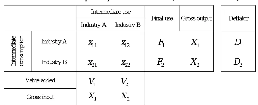
Table 2 presents the output value of each industry X, final demand F, value added V, intermediate transaction between industries x, and deflator for each industry’s output D. DRVA and SRVA denote the production side of real GDP obtained using the double and single deflation methods.
Table 2: Two-sector input–output table and deflator (definition of variables)
The double deflation method subtracts the aggregate of the intermediate consumption for each industry individually deflated from the deflated output value. The production side of real GDP can be determined using the double deflation method as follows:
(4)
Here, we add the real value added of industry A and B.
On the other hand, if full information for the input–output table statistics and precise price indexes are unavailable, an alternative is to use the single deflation method, which directly deflates the nominal value added using the deflator for each industry’s output value. The production side of real GDP by the single deflation method can be obtained using the following equation:
(5)
From the columns of the input–output table, output can be obtained by aggregating intermediate consumption and value added:
Industry A Industry B
Industry A
Industry B
Gross output Deflator
In te rm e d ia te co n su m p tio n Value added Gross input Intermediate use Final use 11
x
x
1221
x
x
221
V
V
21
X
X
21
F
2F
1X
2X
1D
2D
. 2 22 1 12 2 2 2 21 1 11 1 1 D x D x D X D x D x D X DRVA . 2 2 1 1 D V D V(6)
(7)
In addition,
(8)
(9)
When these are assigned to the above single deflation method equation, we get
(10)
The difference between the production side of real GDP obtained from the double and single deflation methods is as follows:
(11)
Therefore, intermediate consumption by itself (x and ) does not affect the results of the single and double deflation methods. Only the intermediate consumption from other industries, which is affected by relative price changes between industries, leads to a divergence between the single and double deflation methods.
Here, we assume that industry A denotes the intermediate industry and industry B the final goods industry. Consequently, We suppose two cases.
Case 1: D1>D2, SRVA<DRVA.
That is, if the price increase in the intermediate goods industries is larger than that in the final goods industries, real GDP determined by the single deflation method is underestimated compared to that estimated using the double deflation method.
Case 2: D1<D2, SRVA>DRVA.
To elaborate, if the price increase in the final goods industries is greater than that in the intermediate goods industries, real GDP determined by the single deflation method is overestimated compared to that obtained using the double deflation method.
We confirm this using a numerical example from the two-sector input–output table.
3-2. Case 1: price rise in the intermediate goods industry is relatively large
Table 3 presents the nominal (left-hand side) and real (right-hand side) input–output tables for the case in which the product prices of industry A (intermediate goods industry) and industry B (final goods industry) increase by 20% and 10% (D1>D2). First, the output value and each demand item of industry A are deflated by 1.20 and those of industry B by 1.10. Then, the aggregate of the realized intermediate consumption is subtracted from the realized output value of each industry, which is the real value added obtained using the double deflation method.
, 1 1 21
11 x V X
x
. 2 2 22
12 x V X
x
), ( 11 21
1
1 X x x
V
). ( 12 22
2
2 X x x
V
In this case, the expenditure (75 + 150 = 225) and production side (115 + 110 = 225) of real GDP are dihedral equivalent.
Table 3: Nominal and real input–output table (price rise in the intermediate goods industry is larger)
Table 4 compares two real value added obtained using the single and double deflation method. Nominal value added of each industry is deflated using output deflators 1.20 and 1.10. It shows that, in this case, production-side real GDP obtained by the single deflation method (117 + 105 = 222) is underestimated compared to that by the double deflation method (SRVA<DRVA) and expenditure-side real GDP.
Table 4: Comparison between single and double deflation method (price rise in the intermediate goods industry is large)
When comparing the deflators, the GDP deflator obtained by the single deflation method (1.15) is larger than that (1.13) using the double deflation method, which is calculated by dividing nominal GDP (255) by real GDP (225). Examining the deflators by industry, for industry B (final goods industries), in which the price rise is relatively low (1.10<1.20), the value added deflator is lower than its production deflator (1.05<1.10). On the other hand, for industry A (intermediate goods industry), in which the price rise is relatively high (1.20>1.10), the value added deflator is higher than the output deflator (1.22>1.20). Thus, the value added deflator by industry has the same direction as the relative magnitude relationship of the output deflator and expands its trend.
3-3. Case 2: price rise in the final goods industry is relatively large
Table 5 shows the nominal (left-hand side) and real (right-hand side) input–output table for the case in which the product price of industry B (final goods industry) increases by 10 percent, but that of industry A (intermediate goods industry) is constant; thus, D2>D1. The output value and each demand item for industry A are deflated by 1.00 and industry B by 1.10 to determine real value added using the double deflation method. In this case as well, the expenditure (90 + 150 = 240) and production side (142 + 98 = 240) of real GDP is dihedral equivalent.
Industry A Industry B Industry A Industry B
Industry A 48 72 90 210 Industry A 40 60 75 175 1.20
Industry B 22 33 165 220 Industry B 20 30 150 200 1.10
70 105 255 430 60 90 225 375
140 115 115 110
210 220 175 200
Value added Value added
Gross input Gross input
Gross
output Deflator
In
te
rm
ed
at
e
co
n
su
m
p
ti
o
n
In
te
rm
ed
ia
te
co
n
su
m
p
ti
o
n
Total Total
Nominal input–output table Real input–output table
Intermediate use
Final use
Gross output
Intermediate use
Final use
Value added of industry A
Value added of
industry B GDP
Real value obtained by the double deflation method 115 110 225
Deflator in case of the double deflation method 1.22 1.05 1.13
Real value obtained by the single deflation method 117 105 222
Table 5: Nominal and real input–output tables (price rise in the final goods industry is large)
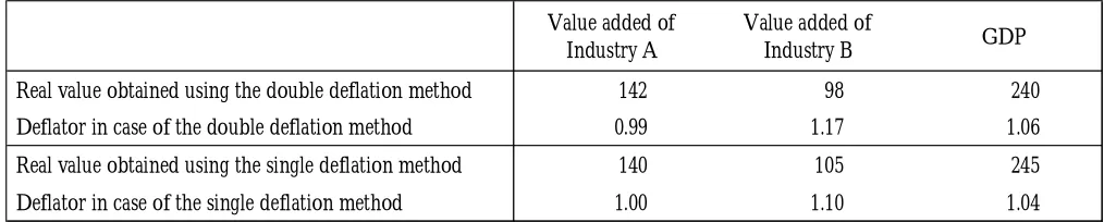
Table 6 is a comparison of real value added obtained using the single and double deflation methods. It can be seen that the production side of real GDP obtained using the single deflation method (140 + 105 = 245) is overestimated compared to the expenditure side of real GDP by the double deflation method (SRVA>DRVA).
When comparing the deflators, the GDP deflator obtained by the single deflation method (1.04) is smaller than that by the double deflation method (1.06). In addition, when drawing a comparison by industry, in industry B (final goods industry), where the price rise is relatively high (1.10>1.00), the value added deflator is larger than the output deflator (1.17>1.10). In industry A (intermediate goods industry), in which the price rise is relatively low (1.00<1.10), the value added deflator is smaller than the output deflator (0.99<1.00). In other words, the value added deflator by industry has a tendency to amplify the relative relationship with the output deflator.
Table 6: Comparison between single and double deflation method (price rise in the final goods industry is large)
4. Verification using Japan’s input–output tables with fixed prices
In Japan, input–output tables include more than 400 sectors at the current price. In addition, since 1960, the linked input–output tables with fixed prices have been created using domestic good, import price, and export price indexes for the 400 sectors.
In this section, we verify the results presented in the previous sections using data from the linked input– output tables for 1960, 1965, and 1970; 1970, 1975, and 1980; 1980, 1985, and 1990; and 1990, 1995, and 2002, which have been co-created by ministries and agencies including the Statistics Bureau of the Ministry of Internal Affairs and Communications. We examine how the prices of the intermediate and final goods industries have changed owing to the economic growth between 1960 and 2000 and whether real GDP determined using the single and double deflation methods are overestimated or underestimated.
Industry A Industry B Industry A Industry B
Industry A 48 72 90 210 Industry A 48 72 90 210 1.00
Industry B 22 33 165 220 Industry B 20 30 150 200 1.10
70 105 255 430 68 102 240 410
140 115 142 98
210 220 210 200
Value added Value added
Gross input Gross input
Gross
output Deflator
In
te
rm
ed
at
e
co
n
su
m
p
ti
o
n
In
te
rm
ed
ia
te
co
n
su
m
p
ti
o
n
Total Total
Nominal input–output table Real input–output table
Intermediate use
Final use
Gross output
Intermediate use
Final use
Value added of Industry A
Value added of
Industry B GDP
Real value obtained using the double deflation method 142 98 240
Deflator in case of the double deflation method 0.99 1.17 1.06
Real value obtained using the single deflation method 140 105 245
In the linked input–output tables, the latest point in time is considered a reference year and the price for the past year, which is the comparison year, is inflated at fixed price; however, in this study, according to GDP statistics convention, the past point in time is the reference year and the price for the new comparison year at fixed price is obtained by deflating it using the reference year price.
In addition, as shown in the previous section, the intermediate demand by itself does not affect the real GDP obtained using the single and double deflation methods. Therefore, when determining the character of the intermediate and final goods industries, we use the intermediate demand rate, excluding intermediate demand by itself.
4-1. Comparison with the 1960–1970 period of high economic growth
During 1960–1970, fixed price increased by an average 4.1% and the Japanese economy underwent tremendous growth, with an average annual rate of 8.6%. Table 7 shows that the average intermediate demand rate, excluding intermediate demand by itself, is 45%. Industries whose rate is higher than the average are considered intermediate goods industries (indicated by ■); industries whose characteristics strongly represent those of the intermediate goods industry are indicated as ■■. Most of the primary and secondary industries are intermediate goods industries and a majority of the tertiary industry falls under the final goods industry category (shown as ●). Industries whose characteristics strongly represent those of the final goods industry are denoted as ●●.
Examining the relative change in price levels between industries, the values for almost all industries are significantly lower than the average inflation rate for the intermediate goods industries (4.1%), except business services; financial and insurance; and agriculture, forestry, and fishery. On the other hand, the prices for the final goods industries are greater than the average, except in the case of machinery and textile industries, which are relatively low as a whole.
Therefore, this period is applicable to case 2 (D1<D2, SRVA>DRVA). That is, since the price increase for the final goods industries is significantly higher than that for the intermediate goods industries, the annual average real GDP growth rate of 11.8% obtained using the single deflation method is largely overestimated than that obtained by the double deflation method (8.6%) (Table 7).
4-2. Comparison with the 1970–1980 period of stable economic growth
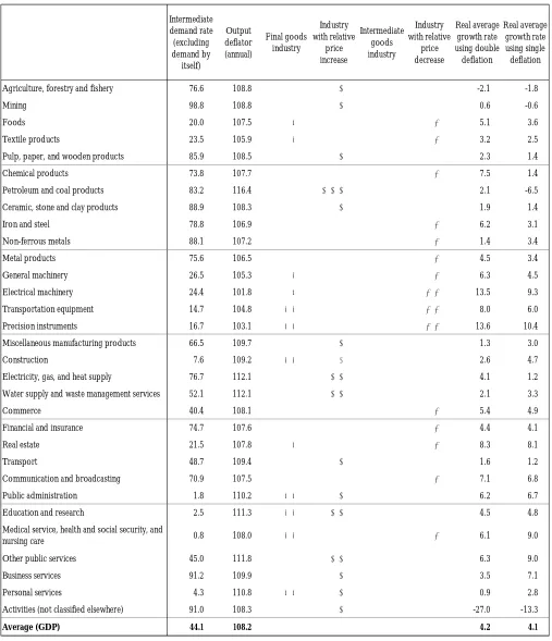
The period of 1970–1980, which encountered the two oil shocks, shows a stable growth in price rise. As shown in Table 8, there is no significant change from the previous period’s average for the intermediate demand rate, excluding that by itself (44.1%); the distribution of the intermediate and final goods industries is also similar. By contrast, part of tertiary industry—water supply and waste management services, transport, and other public services—is observed to have characteristics that strongly represent those of the intermediate goods industries.
Table 7: Comparison of value added between single and double deflation(1960–1970)
Intermediate demand rate (excluding demand by itself)
Output deflator (annual)
Final goods industry
Industry with relative
price increase
Intermediate goods industry
Industry with relative
price decrease
Real average growth rate using double deflation
Real average growth rate using single deflation
Agriculture, forestry and fishery 74.8 106.7 ▲ ■■ -1.3 1.3
Mining 97.9 101.4 ■■ ▼▼ 8.4 8.1
Foods 19.9 104.5 ●● ▲ 5.5 6.6
Textile products 19.1 103.0 ●● ▼ 4.3 9.3
Pulp, paper, and wooden products 83.4 104.0 ■■ ▼ 10.8 13.1
Chemical products 69.3 98.7 ■ ▼▼▼ 21.5 18.4
Petroleum and coal products 85.3 100.7 ■■ ▼▼ 13.4 15.3
Ceramic, stone and clay products 88.9 102.3 ■■ ▼ 14.4 14.8
Iron and steel 80.6 99.7 ■■ ▼▼ 18.0 16.6
Non-ferrous metals 99.4 103.3 ■■ ▼ 8.1 12.1
Metal products 71.1 101.5 ■■ ▼▼ 18.3 19.6
General machinery 23.1 101.2 ● ▼▼ 18.6 17.6
Electrical machinery 27.1 100.9 ● ▼▼ 22.1 19.6
Transportation equipment 22.5 101.5 ● ▼▼ 16.4 17.9
Precision instruments 26.7 103.2 ● ▼ 15.0 15.5
Miscellaneous manufacturing products 61.7 100.8 ■ ▼▼ 17.6 17.7
Construction 11.6 104.3 ●● ▲ 9.7 14.8
Electricity, gas, and heat supply 74.1 103.1 ■■ ▼ 3.3 10.5
Water supply and waste management services 40.2 107.9 ▲▲ 9.5 12.4
Commerce 41.1 103.1 ▼ 15.6 14.8
Financial and insurance 59.5 109.9 ▲▲ ■ 7.4 9.0
Real estate 21.9 109.1 ● ▲▲ 7.6 8.6
Transport 44.5 103.9 ▼ 11.4 11.2
Communication and broadcasting 76.0 102.9 ■■ ▼ 13.4 13.4
Public administration 0.0 111.2 ●● ▲▲▲ -0.2 -0.2
Education and research 0.0 112.3 ●● ▲▲▲ -0.7 2.6
Medical service, health and social security, and
nursing care 0.0 106.3 ●● ▲ -0.5 9.9
Other public services 26.6 109.1 ● ▲▲ -0.7 4.4
Business services 96.2 105.2 ▲ ■■ 8.8 13.8
Personal services 1.4 107.2 ●● ▲▲ 6.7 10.6
Activities (not classified elsewhere) 86.1 102.3 ■■ 24.2 21.5
Table 8: Comparison of value added between single and double deflation (1970–1980)
Intermediate demand rate (excluding demand by itself)
Output deflator (annual)
Final goods industry
Industry with relative
price increase
Intermediate goods industry
Industry with relative
price decrease
Real average growth rate using double deflation
Real average growth rate using single deflation
Agriculture, forestry and fishery 76.6 108.8 ▲ ■■ -2.1 -1.8
Mining 98.8 108.8 ▲ ■■ 0.6 -0.6
Foods 20.0 107.5 ● ▼ 5.1 3.6
Textile products 23.5 105.9 ● ▼ 3.2 2.5
Pulp, paper, and wooden products 85.9 108.5 ▲ ■■ 2.3 1.4
Chemical products 73.8 107.7 ■■ ▼ 7.5 1.4
Petroleum and coal products 83.2 116.4 ▲▲▲ ■■ 2.1 -6.5
Ceramic, stone and clay products 88.9 108.3 ▲ ■■ 1.9 1.4
Iron and steel 78.8 106.9 ■■ ▼ 6.2 3.1
Non-ferrous metals 88.1 107.2 ■■ ▼ 1.4 3.4
Metal products 75.6 106.5 ■■ ▼ 4.5 3.4
General machinery 26.5 105.3 ● ▼ 6.3 4.5
Electrical machinery 24.4 101.8 ● ▼▼ 13.5 9.3
Transportation equipment 14.7 104.8 ●● ▼▼ 8.0 6.0
Precision instruments 16.7 103.1 ●● ▼▼ 13.6 10.4
Miscellaneous manufacturing products 66.5 109.7 ▲ ■ 1.3 3.0
Construction 7.6 109.2 ●● ▲ 2.6 4.7
Electricity, gas, and heat supply 76.7 112.1 ▲▲ ■■ 4.1 1.2
Water supply and waste management services 52.1 112.1 ▲▲ ■ 2.1 3.3
Commerce 40.4 108.1 ▼ 5.4 4.9
Financial and insurance 74.7 107.6 ■ ▼ 4.4 4.1
Real estate 21.5 107.8 ● ▼ 8.3 8.1
Transport 48.7 109.4 ▲ ■ 1.6 1.2
Communication and broadcasting 70.9 107.5 ■■ ▼ 7.1 6.8
Public administration 1.8 110.2 ●● ▲ 6.2 6.7
Education and research 2.5 111.3 ●● ▲▲ 4.5 4.8
Medical service, health and social security, and
nursing care 0.8 108.0 ●● ▼ 6.1 9.0
Other public services 45.0 111.8 ▲▲ ■ 6.3 9.0
Business services 91.2 109.9 ▲ ■■ 3.5 7.1
Personal services 4.3 110.8 ●● ▲ 0.9 2.8
Activities (not classified elsewhere) 91.0 108.3 ▲ ■■ -27.0 -13.3
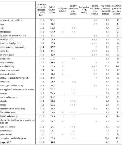
Table 9: Comparison of value added between single and double deflation (1980–1990)
Intermediate demand rate (excluding demand by itself)
Output deflator (annual)
Final goods industry
Industry with relative
price increase
Intermediate goods industry
Industry with relative
price decrease
Real average growth rate using double deflation
Real average growth rate using single deflation
Agriculture, forestry and fishery 73.6 101.2 ■ ▼▼ 1.0 1.5
Mining 100.0 95.7 ■■ ▼▼ -0.6 -1.4
Foods 21.3 113.8 ● ▲▲ -0.9 3.3
Textile products 19.8 114.9 ●● ▲▲ 0.6 2.1
Pulp, paper, and wooden products 79.6 97.2 ■ ▼▼ 3.4 4.7
Chemical products 72.1 78.8 ■ ▼▼▼ 9.8 8.4
Petroleum and coal products 74.9 57.8 ■ ▼▼▼ 8.0 9.4
Ceramic, stone and clay products 89.4 107.7 ■■ ▼ 2.2 3.9
Iron and steel 88.4 81.5 ■■ ▼▼▼ 2.4 3.1
Non-ferrous metals 87.9 82.9 ■■ ▼▼▼ -0.3 5.2
Metal products 88.3 117.4 ▲▲ ■■ 1.8 4.9
General machinery 14.7 106.6 ●● ▼ 7.5 8.0
Electrical machinery 17.9 77.9 ●● ▼▼▼ 15.4 12.6
Transportation equipment 10.4 96.1 ●● ▼▼ 5.8 4.5
Precision instruments 14.2 90.2 ●● ▼▼ 6.7 5.5
Miscellaneous manufacturing products 68.2 104.0 ■ ▼ 4.8 6.0
Construction 7.3 116.9 ●● ▲▲ 4.3 4.8
Electricity, gas, and heat supply 69.8 90.4 ■ ▼▼ 5.5 7.4
Water supply and waste management services 53.3 133.7 ▲▲▲ ■ 2.8 4.1
Commerce 34.6 124.8 ● ▲▲ 2.3 2.7
Financial and insurance 69.2 104.7 ■ ▼ 6.7 6.0
Real estate 20.4 138.8 ● ▲▲▲ 2.2 2.7
Transport 48.2 123.2 ▲▲▲ ■ 2.3 3.8
Communication and broadcasting 67.0 100.5 ■ ▼▼ 6.3 6.0
Public administration 1.4 129.3 ●● ▲▲▲ 0.8 1.5
Education and research 33.0 118.5 ● ▲▲ 4.2 4.4
Medical service, health and social security, and
nursing care 0.0 108.2 ●● ▼ 0.3 4.9
Other public services 25.3 124.1 ● ▲▲▲ -0.4 0.2
Business services 88.0 120.1 ▲▲ ■■ 7.0 8.1
Personal services 3.5 131.2 ●● ▲▲▲ 3.7 4.8
Activities (not classified elsewhere) 83.8 115.0 ▲▲ ■■ 12.6 15.5
Table 10: Comparison of value added between single and double deflation (1990–2000)
Intermediate demand rate (excluding demand by itself)
Output deflator (annual)
Final goods industry
Industry with relative
price increase
Intermediate goods industry
Industry with relative
price decrease
Real average growth rate using double deflation
Real average growth rate using single deflation
Agriculture, forestry and fishery 66.5 92.9 ■ ▼▼ -1.7 -1.8
Mining 100.0 95.4 ■■ ▼ -4.2 -5.0
Foods 20.5 96.3 ● ▼ 1.2 2.0
Textile products 24.8 95.7 ● ▼ -8.1 -6.0
Pulp, paper, and wooden products 86.0 97.6 ■■ ▼ -3.1 -1.7
Chemical products 69.0 86.3 ■ ▼▼▼ 1.3 0.4
Petroleum and coal products 68.6 96.6 ■ ▼ 2.1 2.7
Ceramic, stone and clay products 89.0 98.9 ▲ ■■ -2.7 -1.7
Iron and steel 85.4 70.9 ■■ ▼▼▼ 0.1 -0.1
Non-ferrous metals 81.6 76.8 ■■ ▼▼▼ 0.7 1.8
Metal products 89.9 95.6 ■■ ▼ -3.1 -1.5
General machinery 13.0 97.7 ●● ▼ -2.3 -1.5
Electrical machinery 14.6 72.7 ●● ▼▼▼ 5.1 3.0
Transportation equipment 12.7 96.9 ●● ▼ -1.6 -0.3
Precision instruments 15.9 95.4 ●● ▼ -3.0 -1.8
Miscellaneous manufacturing products 69.5 102.6 ▲▲ ■ -2.7 -0.7
Construction 11.4 104.1 ●● ▲▲ -2.4 -1.6
Electricity, gas, and heat supply 67.6 82.6 ■ ▼▼▼ 4.9 3.7
Water supply and waste management services 62.3 116.1 ▲▲▲ ■ 0.0 1.0
Commerce 34.4 98.1 ● ▲ 2.0 2.0
Financial and insurance 69.5 87.7 ■ ▼▼▼ 2.6 2.2
Real estate 13.3 114.4 ●● ▲▲▲ 2.1 2.3
Transport 45.5 98.4 ▲ ■ 1.2 1.2
Communication and broadcasting 58.8 88.4 ■ ▼▼ 6.9 6.4
Public administration 2.6 105.0 ●● ▲▲ 3.0 3.3
Education and research 34.3 110.9 ● ▲▲▲ 1.3 1.7
Medical service, health and social security, and
nursing care 0.0 105.1 ●● ▲▲ 4.8 5.6
Other public services 24.9 108.3 ● ▲▲▲ -0.5 -0.2
Business services 74.8 106.1 ▲▲ ■ 2.9 3.4
Personal services 4.6 113.0 ●● ▲▲▲ -0.9 0.2
Activities (not classified elsewhere) 98.7 98.8 ▲ ■■ -7.3 -6.6
The intermediate goods industries excepting these industries showed a relative price decrease for the period of 1960–1970. In addition, the final goods industries depict similar patterns, with the machinery, textile products, and food industries showing price declines, whereas education, research, and personal services reporting a price rise.
In other words, in this period, the intermediate and final goods industries are affected by conflicting elements, and therefore, a significant trend is not observed in the relative price change for the 1960–1970 period. As a result of this offset, the GDP growth rate of 4.1% obtained using the single deflation method reaches closer to the growth rate of 4.2% by the double deflation method.
4-3. Comparison with the 1980–1990 period of stable growth
In 1980–1990, stable growth continued under the growing inflation rate. As shown in Table 9, although the mean of the intermediate demand rate, excluding that by itself dropped to 38.8%, the distribution of the intermediate and final products industries is almost the same as that in the previous period.
We now analyze the relative change in price levels between the industries. In comparison to the average inflation rate of 8.3%, among the intermediate goods industries, except business services and metal products, which have strong intermediate goods characteristics, the price increase for most industries are well below the average rate. On the other hand, in the final goods industry, as a whole, the price increase for the industries is much higher than the average, except in the case of machinery industries, whose price levels showed a relative decrease.
Therefore, this period, as well as 1960–1970, is notably applicable to case 2: D1 <D2, SRVA >DRVA. That is, as a whole, since the price increase in the final goods industries is much higher than that in the intermediate goods industries, the average real GDP growth rate of 5.1% obtained from the single deflation method is significantly overestimated than that by the double deflation method (4.2%) (Table 9).
4-4. Comparison with the 1990–2000 period of low-growth
Finally, we review the 1990–2000 period of low growth under deflation, that is, after the collapsed of the asset price bubble. As shown in Table 10, while the absolute price level is −2% (deflation), which is the reverse of the price soar in the 1980s, there is a clear trend similar to that of the past relative changes among the industries, that is, a price decrease in the primary and secondary industries and price rise in the tertiary industry. In other words, the relative price of intermediate goods industries reduces as a whole and most of the relative prices in the final goods industries rise.
Therefore, Case 2, D1<D2, SRVA >DRVA, holds true for this period. Despite the low growth of around 1%, it can be seen from Table 10 that the average real GDP growth rate of 1.6% obtained by the single deflation method is overestimated than that by the double deflation method (1.1%).
5. Conclusion
The double deflation method as a quantitative measure of value added is premised on the ideal situation of the availability of complete information in input–output table statistics and precise price indexes. However, in reality, it is often difficult to develop these statistics on an annual or quarterly basis. An alternative, as recommended by United Nation’s SNA, is the single deflation method, which deflates the nominal value added using the output deflator of each industry when full information is unavailable. In other words, it is assumed that in not a long term, there is no significant change in the intermediate consumption or value added rate of each industry and price fluctuations received by value added can be approximated by those in industry output.
We also divided 40-year data (1960–2000) for Japan by four periods. We considered the relative change in the price levels in each industry and compared and analyzed the impact of these changes to the estimation results obtained using the double and single deflation methods. We mainly found the following trends.
First, the primary industry and most of the secondary industry, except the mechanical industries, have characteristics that strongly represent those of the intermediate goods industry. On the other hand, most of the tertiary industry, except the business services, can be categorized as the final goods industry. Next, for relative change in the price levels between the industries, we found that, except during 1970–1980, when the oil shocks occurred, the product prices of the primary and secondary industries relatively decreased and those of the tertiary industry increased owing to the rise in labor factor prices. Therefore, as a whole, the price of the intermediate goods industry showed a declining trend and that of the final goods industry tended to increase. As a result, we suggest that the real economic growth rate estimated using the single deflation method is likely to be overestimated.
Acknowledgement: This Works was supported by the Grant-in-Aid for Scientific Research (C) of 2015 (Project
Number 23530247).
References
ESRI (2007) SNA estimation method manual (2007 revised edition). [Online]
Available: http://www.esri.cao.go.jp/jp/sna/data/reference1/h12/sna_kaisetsu.html (in Japanese). ESRI (2012) SNA estimation method manual (Annual estimates, eds., 2005 standards version). [Online]
Available:http://www.esri.cao.go.jp/jp/sna/data/reference1/h17/pdf/kaisetsu20121116.pdf(in Japanese). NBS (2008) China non-economic census annual GDP calculation methods, China Statistics Press (in Chinese). United Nations (1968) System of National Accounts. [Online]
Available: http://unstats.un.org/unsd/nationalaccount/docs/1968SNA.pdf. United Nations (1993) System of National Accounts 1993. [Online]
Available: http://unstats.un.org/unsd/nationalaccount/docs/1993sna.pdf. United Nations (2009) System of National Accounts 2008. [Online]