QUANTIFICATION AND INCORPORATION OF UNCERTAINTY
IN FOREST GROWTH AND YIELD PROJECTIONS USING A
BAYESIAN PROBABILISTIC FRAMEWORK
(A DEMONSTRATION FOR PLANTATION COASTAL DOUGLAS-FIR IN THE PACIFIC
NORTHWEST, USA)
Duncan Wilson
1, Vicente Monleon
2, Aaron Weiskittel
31Oklahoma State University, Department of Natural Resource Ecology & Management, Stillwater, OK, USA, 74078 2USDA Forest Service, PNRS, FIA Program, Corvallis, OR, USA, 97331
3University of Maine, Center for Research on Sustainable Forests, Orono, ME, USA, 04469
Abstract.A Bayesian probabilistic modeling platform was used and evaluated for application in a relatively complex individual-tree growth and yield model for coastal Douglas-fir (Pseudotsuga menziesii
var. menziesii (Mirb.) Franco), which was expressed as a mixed discrete and continuous Bayesian Network for annual projections. The modeling platform used a common and open-source Bayesian analysis program (JAGS v3.3.0), and was sufficiently flexible to handle a relatively complex model structure; namely, a dif-ferential form, highly dynamic, recursive, hierarchical, non-linear system of equations with rather complex error structures. This novel probabilistic modeling platform met certain desirable criteria, including: (1) accurate and tractable projections that included full error propagation; (2) flexible and comprehensive analytic capabilities; (3) full consideration of hierarchical and multi-level model structures; (4) capacity for random effects calibration; (5) allowance of hypothesis testing and updating knowledge across different system components, simultaneously with varying sources of information (i.e., new data); (6) computational efficiency; and (7) relatively simple implementation as demonstrated in a compiled scripting language. Probabilistic projections of forest growth and yield included all sources of errors and uncertainty (e.g., estimated parameters, state variables, random effects, and residual errors). Cumulative error projections over a 40-year period for three sample Douglas-fir stands were determined. Projection errors for key metrics summed across all trees, such as total basal area and stem density, had coefficient of variations between 4-6% and 7-8%, respectively. Probabilistic projections were markedly different from deterministic projections made with the same model structure. Overall, this novel probabilistic platform showed strong promise as a general platform for ecological modeling, particularly when tractable and analytically correct error projections are required. In particular, the Bayesian probabilistic modeling approach used provided a natural platform for cross-disciplinary research, particularly between social and ecological research domains.
Keywords: forest growth and yield, error propagation, model uncertainty, error budgets, individ-ual tree growth models, coastal Douglas-fir, Oregon, Washington.
1
Introduction
Ecological modeling is dominated by deterministic ap-proaches, particularly in forestry (Canham et al. 2003, Weiskittel et al. 2011). The structure of the modeling equations is dependent on the system being modeled as well as the objectives, and so it varies considerably be-tween published models. Such models are ubiquitous in ecological research, with examples ranging from
pro-jecting animal and plant meta-population dynamics, to process-level vegetation growth, food chains, plant suc-cession and migration, and disturbance risk, as well as social and economic dynamics linked to ecological pro-cesses (An 2012). Notably, we do not include agent-based models (Epstein 2006) or models of purely phys-ical processes (e.g., fire dynamics or weather), which can be viewed as more stochastic implementations. In contrast, most ecological models take a difference
tion approach with a discrete time or spatial step, al-though systems of differential equations are not uncom-mon (Arnold et al. 1998). While many ecological models incorporate stochastic elements (e.g., weather, mortality events), these discrete elements are usually embedded within an otherwise deterministic framework.
Forest growth and yield (GY) models have a long history of development and are prime examples within a field dominated by difference-form, deterministic approaches (Pienaar and Shiver 1986, Weiskittel et al. 2011). The current challenges in forest GY mod-eling serve as an illustration for the broader field of ecological modeling. Forest GY models are ubiquitous in forestry, with particular use in economic forecasting, designing silvicultural systems, risk management, har-vest scheduling, forecasting fiber supply, carbon dynam-ics, and ecosystem management (LeMay and Marshall 2001). The structure of forest GY models vary, but the majority were designed as a system of equations that sequentially predict structural attributes from inventory data and variables previously projected by the model. Forest GY models have variable time steps, but an an-nual interval is often preferred for a variety of reasons (Weiskittel et al. 2011). Similar to temporal resolu-tion, forest GY models can also have different spatial resolutions ranging from individual trees to stand at-tributes with increasing focus on higher spatial resolu-tions (Weiskittel et al. 2011). Consequently, individ-ual tree-level models with an annindivid-ual temporal resolu-tion have become the primary focus for both research and practical implementation (e.g., Kershaw et al. 2017; Weiskittel et al. 2016a, 2017).
Within a forest GY model, a variety of component equations that sequentially predict tree- or stand-level attributes (e.g., tree diameter or live stem density) are used. Most often, these equations are fitted indepen-dently and then sequentially linkedpost hoc. The com-ponent equations are also often strongly non-linear, and may have correlated residuals across component tions. While simultaneously modeling systems of equa-tions to account for correlated errors has been used in this past (e.g., Hall and Clutter 2004), this method is usually used only for a subset of the equations. As a consequence, estimates of prediction error are generally lacking due to the complexity of the system of equa-tions. In fact, most forest GY models provide no esti-mate of projection uncertainty and relatively few studies have attempted to address this for forest management– orientated models (e.g., Gertner et al. 1996; Green et al. 1999; MacFarlane et al. 2000; McGarrigle et al. 2013; Kershaw et al. 2017).
Furthermore, ecosystem management has progressed to the point where traditional forest GY projections of total volume or diameter distributions are no longer
suf-ficient (McComb et al. 1993). Many ecosystem dynam-ics and structural elements are highly stochastic both temporally and spatially. Consequently, they are often not very well represented within a deterministic model-ing framework. An example is modelmodel-ing the understory vegetation composition and dynamics that are an impor-tant habitat component for many small mammals and songbirds (Wilson and Puettmann 2007). Vegetation re-sponse to thinning is strongly tied to pre-treatment con-ditions, which are highly variable and largely unrelated to current overstory conditions (Wilson et al. 2009). As such, modeling vegetation within existing forest GY models becomes extraneous when vegetation predictions are largely independent of tree growth. Many simi-lar information needs for ecosystem management sim-ply do not fit within the current GY framework and, as a result, such modeling efforts have progressed inde-pendently (e.g., Running and Gower 1991, Scheller et al. 2007) rather than collaboratively.
In this study, we highlight the utility of a probabilistic modeling platform for addressing many of the challenges common to ecological models. We re-parameterized an individual-tree GY model (DF.GOAB) for plantation-grown, coastal Douglas-fir (Pseudotsuga menziesii
(Mirb.) Franco var. menziesii; Weiskittel et al. 2007) to demonstrate the advantages of this approach. The model platform is a continuous-node form of a Bayesian Network (Pearl 1988) that we updated (i.e., projected) using current tree- and stand-level structural informa-tion along with Bayes’ theorem. The results are pre-sented as posterior distributions, which are computed numerically with a Markov Chain Monte Carlo (MCMC) sampling approach. Unlike deterministic models, updat-ing the model is efficient with stochastic elements, which can exponentially increase the computational require-ments. Component equations, such as dominant height growth or mortality, are ideally developed using con-temporary Bayesian parameter estimation approaches (Gelman et al. 2013), but this is not a strict require-ment. These component equations can take almost any form, including continuous or discrete, linear and non-linear functions or distributional states. Error structures can include Gaussian and other exponential families, but also non-standard user-defined distributions, as well as hierarchical structures. Similar approaches to quanti-fying uncertainty using a Bayesian approach have been previously demonstrated in other disciplines (e.g., Freni and Mannina 2010) yet remain uncommon in forest sci-ence.
plat-form is quite general, so we do not attempt to fully present here the model details or assess prediction ac-curacy with independent data. Instead, our primary objective is to contrast the probabilistic approach with current practices (i.e., deterministic and quasi-stochastic modeling approaches). We also will demonstrate several instances where deterministic and probabilistic models potentially have different projections. First, we present the probabilistic modeling platform and how projections are made, and then how the revised DF.GOAB model is portrayed in a Bayesian Network.
2
Methods
2.1 Bayesian probabilistic modeling platform
The Douglas-fir GY modeling system we chose to il-lustrate this approach is typical for this class of mod-els, and representative of approaches taken in many ter-restrial vegetation dynamics models. The component equations are a mixture of linear and non-linear equa-tions, with weighting and multiple hierarchical random effects, and have a discrete time-step. In deterministic approaches, the estimated equation parameters are typ-ically fixed at the value of their point estimates, often with some level of stochasticity to predict categorical variables such as mortality. Most systems of equations, including the ones in this study, are highly recursive, with predicted variables used as predictors in subsequent time-steps. These approaches ignore the uncertainty in the estimation of both parameters and predicted vari-ables, and the stochastic component of the models equa-tions (Dennis et al. 1985). To address these issues, the system of equations used in the study was fitted to an existing database of Douglas-fir growth, and then por-trayed in a Bayesian probabilistic modeling platform. We used a mixed categorical- and continuous-node form of a Bayesian Network (Pearl 1988, Nielsen and Jensen 2009).
There is a large literature on contemporary Bayesian parameter estimation, and since the model projections follow the same methodology, we focus our explana-tion on where the applicaexplana-tions (parameter estimaexplana-tion versus model projections) differ. Models are expressed similarly in both Bayesian Networks and in contempo-rary Bayesian parameter estimation as directed acyclic graphs (DAG; Nielsen and Jensen 2009). This approach allows very complex models, including hierarchical mod-els and systems of equations, to be expressed as a se-ries of conditional distributions defined in a parent-child relationship (Wikle 2003). Specifically, the full, joint probability distribution for the entire model can be written as the product of conditional distributions, P(x1, ..., xn) = Πni=1P(xi|pa(xi)), where, xi is the full
suite of variables, and pa(xi) represents the parents of
xi. This relatively simple factorization allows complex
models to be described through simpler marginal prob-abilities, and thus estimate individual components sep-arately, while retaining connectivity throughout the en-tire model.
Models in a Bayesian framework for both parameter estimation and model projections take the same gen-eral form in that parameters are represented as random variables with an associated prior probability distribu-tion, with the model structure expressing the form of the likelihood. The contrast between Bayesian parameter es-timation and model projections in a Bayesian Network are: (1) parameters in a Bayesian Network are expressed as highly informative priors with means and standard er-rors for the parameters usually taken from fitted equa-tions and (2) the Bayesian Networks do not necessarily include new data to update the priors. Projections are made for “child” variables based on parent-child hierar-chy (i.e., model structure), which is expressed as a series of conditional probabilities defined by the DAG. These generally include state variables as well as parameters estimates and all sources of error. Posterior distribu-tions for projected variables are computed numerically with a Markov Chain Monte Carlo (MCMC) sampling approach since most model forms do not have a closed-form analytical solution. This MCMC approach to a Bayesian Network is not a traditional discrete-state type but is more a type of efficient random-walk first toward and then within the stable posterior distribution (Capp´e and Robert 2000). The MCMC approach is automati-cally contained within the stable posterior distribution when no new data are included.
Model projections without new data are essentially infilling of “missing” model response data, where pro-jections of tree- and stand-level variables over time (as in our study) represent these missing data. If some of this data becomes available, it can be provided to the model, which allows for simultaneous updating of model parameters (e.g., random effect calibration, state or la-tent variable estimation, etc.). Also, different types of new data will update different model parameters (in-cluding error parameters) depending on the structure of the model (Wilson et al. 2009) because systems of equa-tions are represented simultaneously in Bayesian Net-works. Here, we describe projections as missing data to underscore how projected responses from the model are conditionally related to the model parameters and state variables.
the lines between the two approaches (Clark and Gelfand 2006, Wilson et al. 2009). Within the Bayesian Network, projections are made for each tree over each projection year. This projection on an “annual time step” is a slight misnomer in a Bayesian Network since each iteration of the Markov chain updates every tree for every year in the projection. Thus, 1,000 MCMC iterations does not represent a 1,000 year projection, but rather 1,000 sam-ples from the posterior distribution, with each sample containing a full set of projections for every tree and year combination. The MCMC iterations collected for each variable comprise the marginal posterior distribu-tions. For simplicity, the model parameters, residuals, and prior distributions are all assumed to be uniformly normal in this analysis. This assumption might be im-portant as some of the parameters and residuals may not be normally distributed given the complex non-linearity of the models used. In addition, the wrong prior distri-bution can lead to incorrect estimations of uncertainty in modeling results (Freni and Mannina 2010).
2.2 Dataset
Data from 65 University of Washington Stand Man-agement Cooperative permanent research installations in Oregon and Washington, USA, and Vancouver Is-land, British Columbia, Canada were used for analy-sis. These installations cover a wide range of growing conditions typical of the region. The overall climate is humid oceanic, with a distinct dry summer and a cool, wet winter. The twenty-year mean annual rainfall for these locations ranged from 91 to 293 cm (18–32% oc-curring during the growing season), and January and July mean temperatures ranged from -2.7 to 6.7°C and 14.7 to 19.2°C, respectively. Variation in precipitation and temperature are strongly related to elevation and distance from the coast. Elevation ranged from 5 to 1160 m above sea level, slope was between 0 and 60%, and all aspects were represented. Soils varied from a moderately-deep sandy loam to a very deep clay loam with mean water holding capacity of 139±63 mm (45 – 303 mm).
Since its establishment in 1985, the Stand Manage-ment Cooperative (SMC) at the University of Wash-ington (http://www.cfr.washWash-ington.edu/research.smc/) has maintained a database representing 435 installations in British Columbia, Washington, and Oregon (Maguire et al., 1991). In this study, we focus on a subset of these data, restricted to pure, plantation-grown Douglas-fir in western Oregon, Washington, and British Columbia; specifically, Douglas-fir plantations extracted from the Type I, II, and III installations. Type I installations are square 0.2 ha plots established in existing plantations that have received designed sets of silvicultural
treat-ments since plot establishment in the late 1980s and early 1990s. Type II installations are square 0.2-ha plots that were installed between 1986 and 1991 in stands ap-proaching commercial thinning age and received differ-ent levels of commercial thinning treatmdiffer-ents. Type III installations were established between 1985 and 1990 as initial spacing trials with six densities ranging from 247 to 3048 trees per ha. Plot size for Type III installations varied from 0.086 ha at the highest density to 0.202 ha at the lowest density. For this analysis, only the untreated (i.e., control) plots in the Type I, II and III installations were used, resulting in a model fitting database of 167 plots across 65 installations.
At each plot, individual trees were tagged and mea-sured for diameter at breast height (D) with a subsam-ple of trees measured for total height (HT) and height to crown base (HCB). Common variable definitions and abbreviations are given in Table 1. Plots were generally re-measured on a 4-year interval (range 2-8 yrs; Table 2). A subsample of trees were measured for HT and HCB on each plot, but with the exception of estimating missing heights to compute dominant height (HD), only directly measured variables were used in equation fitting.
2.3 Growth and yield equations
Forest GY models have a long tradition of develop-ment and use in forestry (Weiskittel et al. 2011). They are designed to project tree- or stand-level growth over time beginning with a discrete starting condition, often taken from a field-measured inventory. These models are fundamentally similar to many terrestrial vegetation and wildlife models, different only in the model focus (tree growth, soil organic matter, wildlife populations size, etc.) and data describing starting conditions.
We modified a previously published system of equa-tions developed to project GY of individual Douglas-fir trees on an annual time-step (DF.GOAB; Weiskittel et al. 2007). This system of equations was derived from model forms used in the ORGANON-SMC GY model for coastal Douglas-fir (Hann et al. 1993, 2003). Model vari-ables are either measured in a field inventory at the start of the projection (t0), projected for time step t, or
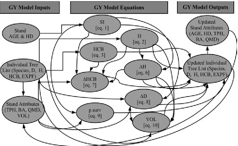
Figure 1: Structure and inter-relationships between model inputs, equations, and outputs for the Douglas-fir growth and yield (GY) model framework used in this analysis.
is then the expected height of the dominant trees at a reference age, taken as 25 years from planting for this study. Dominant height was predicted using a Hossfeld function fitted as a non-linear difference form equation,
SI= Age
2
SI
AgeSI
Age
10
HD10 +α11
+ α10
Age10+
+α11Age10+α10
+SI (1)
where α10 are estimated parameters, Agesi is the site
index age (25 years from planting in this study), Age0 is the breast-height age at the initial inventory, HD0
is the dominant height at the initiation inventory, and residual error is weighted by projection period,εSI∼N.
SI was estimated for each plot and then averaged for an installation.
It is assumed that all trees were measured for the ini-tial diameter, D0 , in the initial inventory. However, H
and HCB were only measured on a subsample of trees. Unmeasured individual tree heights,Hifor treeiat the
start of the projection (t0), were estimated with a power
function and transformed to the log-log scale. This was done for each inventoried plot separately.
ln(Hi0) =β0+β1ln(Di0) +Hi0 (2)
where β0−1 are estimated parameters, and residual
er-rors,H ∼N 0, σH2
specific to a single plot. Similarly, the HCB was estimated using the same model form,
ln(HCBi0) =γ0+γ1ln(Di0) +HCBi0 (3)
where γ0−1 are estimated parameters, and HCB ∼
N 0, σ2
HCB
. The equation predicting maximum crown width (MCW) for open grown Douglas-fir trees was taken directly from Hann (1999) and applied as a known relationship without any incorporation of uncertainty. Similarly, covariates derived from MCW were treated as known.
Projections were made on an annual time step (t) for each tree. Dominant average heightHD of the invento-ried plot was projected using [Eq. 1] modified as,
HD= Age
2
t
Aget
Age
t−1
HDt−1 +α41
+ α40
Aget−1+
+α41Aget−1+α40
+HD (4)
where α40−41 are estimated parameters, and HD ∼
N 0, σ2
HD
. The Hossfeld function based base-age in-variant equation (Cieszewski 2003) was selected because it showed adequate fit to the data and could be alge-braically solved forAget . Growth effective age (GEA) was defined as the expected age of an individual tree for a given height, had that tree followed the dominant height trajectory (Eq. 1) for the plot estimatedSI. For each time step,GEAitwas defined as the algebraic
solu-tion for Aget in Eq. 4 based on substituting AgeSI for Aget−1 ,SI forHDt andHit−1 for HDt−1 . Potential
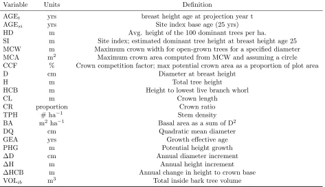
Table 1: Common variable units and definitions used in this analysis.
Variable Units Definition
AGEt yrs breast height age at projection year t
AGEsi yrs Site index base age (25 yrs)
HD m Avg. height of the 100 dominant trees per ha.
SI m Site index; estimated dominant tree height at breast height age 25 MCW m Maximum crown width for open-grown trees for a specified diameter MCA m2 Maximum crown area computed from MCW and assuming a circle
CCF % Crown competition factor; max potential crown area as a proportion of plot area
D cm Diameter at breast height
H m Total tree height
HCB m Height to lowest live branch whorl
CL m Crown length
CR proportion Crown ratio
TPH # ha−1 Stem density
BA m2ha−1 Basal area as a sum of D2
DQ cm Quadratic mean diameter
GEA yrs Growth effective age
PHG m Potential height growth
∆D cm Annual diameter increment
∆H m Annual height increment
∆HCB m Annual change in height to crown base
VOLib m3 Total inside bark tree volume
as,
P HGit=
(GEAit−1+ 1)2
(GEAit−1+ 1)N5+α40
−Hit−1, (5)
where: N5 =
GEAit−1
Hit−1 +α41GEAit−1 −
α40
GEAit−1 +
α2(GEAit−1+ 1).
Individual tree height growth was then modeled as a function of potential height growth, modified to ac-count for stand- and tree-level covariates, similar to Ar-ney (1985) as,
∆Hit =
H
it−1
HDit−1
ψ60+install∆H+plot∆H
×
1−ψ61
CCF
it−1 600
ψ62
×P HGit+∆H
(6)
where ψ60−62 are estimated parameters, install∆H and
plot∆Hare random effects assumed distributed Gaussian
with means zero and variances σ∆2H
install and σ 2 ∆Hplot,
respectively, and residual error is weighted by H as, ∆H∼N 0, Hit2−1σ∆2H
.
Recession in HCB was adapted from Hann and Hanus (2004) as,
∆HCBit=
CLit−1+ ∆Hit
1 + exp (N7) +∆HCB (7) where, N7 = ϕ70 + install∆HCB + plot∆HCB +
ϕ71ln(CRit−1) + ϕ72CRit−1 + ϕ73GEAit−1 +
ϕ74ln(BAit−1) + ϕ75
CRit−1
BAit−1, and where, ϕ70−75
are estimated parameters, CL is crown length, CR is crown ratio, install∆HCB and plot∆HCB are random
effects assumed distributed Gaussian with means zero and variances σ2
∆HCBinstall and σ 2
∆HCBplot,
re-spectively, and residual error is weighted by CL as, ∆HCB∼N 0, CL2it−1σ∆2HCB
.
Diameter growth was adapted from Hann et al. (2006) as,
∆Di= exp
θ80+install∆D+plot∆D
+θ86BA0it.−15 +θ85DQDit−1 it−1
+θ81Dit−1+θ82D2it−1
+θ83ln
CRit−1+0.2 1.2
+θ84ln(SI−1.37)
+∆D (8)
where θ80−86 are estimated parameters, install∆D and
plot∆Dare random effects assumed distributed Gaussian
with means zero and variances σ2
∆Dinstall andσ 2 ∆Dplot ,
respectively, and residual error is weighted as∆DBH ∼
N 0, DBH2it−1σ2 ∆DBH
.
Individual tree survival probability was modeled with logistic regression,
logit(p.survit) = δ90+δ91Dit−1+θ92SI
+θ93
1− Dit−1
DQit−1 +θ94BAt−1
(9)
where δ90−94 are estimated parameters. Crown length
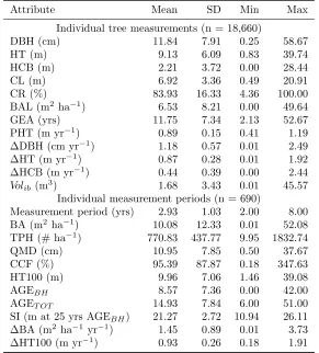
Table 2: Attributes of the individual trees and plots used for constructing the equations.
Attribute Mean SD Min Max
Individual tree measurements (n = 18,660)
DBH (cm) 11.84 7.91 0.25 58.67
HT (m) 9.13 6.09 0.83 39.74
HCB (m) 2.21 3.72 0.00 28.44
CL (m) 6.92 3.36 0.49 20.91
CR (%) 83.93 16.33 4.36 100.00
BAL (m2 ha−1) 6.53 8.21 0.00 49.64
GEA (yrs) 11.75 7.34 2.13 52.67
PHT (m yr−1) 0.89 0.15 0.41 1.19
∆DBH (cm yr−1) 1.18 0.57 0.01 2.49
∆HT (m yr−1) 0.87 0.28 0.01 1.92
∆HCB (m yr−1) 0.44 0.39 0.00 2.44
Volib (m3) 1.68 3.43 0.01 45.57
Individual measurement periods (n = 690)
Measurement period (yrs) 2.93 1.03 2.00 8.00 BA (m2 ha−1) 10.08 12.33 0.01 52.08 TPH (# ha−1) 770.83 437.77 9.95 1832.74
QMD (cm) 10.95 7.85 0.50 37.67
CCF (%) 95.39 87.87 0.18 347.63
HT100 (m) 9.96 7.06 1.46 39.08
AGEBH 8.57 7.36 0.00 42.00
AGET OT 14.93 7.84 6.00 51.00
SI (m at 25 yrs AGEBH) 21.27 2.72 10.94 26.11
∆BA (m2ha−1 yr−1) 1.45 0.89 0.01 3.73
∆HT100 (m yr−1) 0.93 0.26 0.18 1.91
to increase the number of trees available for fitting the model, since most trees were not directly measured for these metrics.
Finally, tree-level attributes like D and H are com-monly used to predict individual tree volume (Vol) so un-certainty in either of these estimates could significantly influence this estimate. Consequently, a volume equa-tion similar in form to Honer et al. (1965) was derived using a subset of destructively sampled Douglas-fir trees (n= 337),
Volib=
D
θ100+θ101H
(10)
whereVolib is the total volume inside bark andθ100−101
are estimated parameters.
Except for the survival as well as H and HCB at t0 equations, all other equations were fitted using the
nlme package (Pinheiro and Bates, 2000) in R v3.0.2 (R Development Core Team, 2012). The increment equa-tions were annualized from multi-year measurement in-terval data using an iterative technique described by Cao (2000) and Weiskittel et al. (2007). All parameters were estimated using nonlinear mixed effects with installa-tion and plot within installainstalla-tion as random effects. Since
these data violated the assumption of homogeneous vari-ance, a power variance function of the primary covariate was incorporated into the fitting function for the equa-tions. The power variance function was common to all installations and plots and was defined in this analysis as s2(v) =|v|(2x), where v is the variance covariate, s2(v)
is the variance function evaluated at v, and x is the vari-ance function coefficient. Missing H and HCB data were fitted directly within the Bayesian model using contem-porary parameter estimation techniques (Fig. 2). The fitted parameters were given non-informative priors as ˜N(0,10000), with the residual errors given partially in-formative priors,σ˜uniform(0,20). Parameter estimates, standard errors, correlation between parameters, as well as residual errors were fitted and directly incorporated into projections in the Bayesian Network.
Table 3: Variable states as inventoried, derived or projected for individual treei or stand level. Variables only used in projections that are set at current values are shown as time step t-1. Recursive variables are those where the current value affects projections are shown in italics.
Source (time step) Variable
Inventory (t0) Di, Hi*, HCBi*, Survi Age Derived (t0) Cli, CRi, HD, SI, BA, TPH, CCF
Projected (t-1) GEA, CCF, BA, TPH
Projected (t) HD, PHG, HMOD, ∆Di, ∆Hi, ∆HCBi, Survival Derived (t) D, H, HCB, CR, CCF, BA, TPH, HD, DQ
Notes: Constants, parameters and transformed variables are not shown.
∗Often only a subsample is measured.
Figure 2: Missing heights were estimated prior to growth projections with two randomly chosen MCMC iterations shown here (circles and triangles). Only a randomly chosen subset of missing heights on plot 1 are shown for clarity. The estimated regression functions for both MCMC iterations are also plotted.
exception that explanatory covariates retained the val-ues at the start of each measurement period. Priors for the parameters were δ1−5 ˜N(0,1000). This Bayesian
model fitting was done separately, and then parameter estimates, standard errors, and correlation between pa-rameters were inputted as data for the Bayesian Network to predict annual survival probabilities.
2.4 Bayesian model projections
To illustrate model projections, inventory data from three Douglas-fir plots were used as starting points in model projections (Table 4). Each plot was pure Douglas-fir, with a full inventory of D and subsampled H and HCB from single 0.202 ha plots. These data were used in a regional GY cross-model comparison (Johnson 2005), so they represented a range of growing conditions
typical for the region and provided a convenient refer-ence.
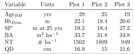
Table 4: Douglas-fir stand characteristics (Breast Height Age, Dominant Height, Site Index, Basal Area, num-ber of trees per ha, and Quadratic Mean Diameter) for three 0.202 ha inventoried plots serving as starting con-ditions for the 40-year model projections. The inventory data is from Johnson (2005) and was available online at www.growthmodel.org.
Variable Units Plot 1 Plot 2 Plot 3
AgeBH yrs 29 25 19
HtDom m 22.1 18.4 20.6
SIa m at 25 yrs 19.2 18.4 27.2
BA m2 ha−1 33.7 31.8 34.8
NT # ha−1 1502 1809 949
QD cm 16.9 15 21.6
a
Eq. 1 estimated.
con-stant for each projection year and tree within that sin-gle iteration. Residual errors, however, were randomly generated for each tree and projection year within a sin-gle MCMC iteration. Residual errors were randomly generated based on the estimated residual errors, but then applied (i.e., added) on the unweighted scale. In-dividual tree survival in a projection year was randomly determined based on the computed mean probability of survival. A few restrictions were added to the model structure such as not allowing D, H, or HCB to decrease with increasing age, although HD was not similarly con-strained. Survival was tracked for individual trees to ensure consistency. Finally, plot average or summation variables such as DQ or TPH were expanded to a per-ha basis and computed within each iteration, and therefore also expressed as posterior densities.
All projections were made with JAGS v3.3.0 (Plum-mer 2003). Each projection started with the inventory list from the three plots. Initial H and HCB were mea-sured on approximately 15% of the plot trees, so these variables were estimated for trees with missing data us-ing equations 2 and 3 embedded within the Bayesian Network. The base projection of 40 years included all sources of error and uncertainty, including a stochasti-cally applied survival function. A fixed random num-ber “seed” was used for repeatability of results. An initial 25,000 MCMC iterations were used as a “burn-in” period, and discarded. Projections were comprised of 40,000 additional MCMC iterations, retaining every 10th iteration to reduce serial correlation. These 4,000 MCMC iterations formed the posterior distributions of the projected variables. Note that this burn-in period and serial correlation concerns were only necessary due to missing H and HCB data being estimated directly within the projection model. Additionally, we randomly chose 25% of these MCMC iterations to illustrate model behavior.
2.5 Error budgets
One of the principal advantages of a Bayesian Net-work is the automatic propagation of errors throughout the model. This is achieved since each variable is con-nected through the conditional relationships depicted by the Bayesian Network. We examined the error budgets of the Douglas-fir GY model by investigating how un-certainty in the component equations (i.e., residual vari-ance, parameter error, random effects, or state uncer-tainty) influenced system-wide error. Forty-year projec-tions were made for each of the three plots that included all errors (i.e., base projection), where all errors were set to null values (i.e., a deterministic model with all errors set to zero), and finally, where individual error terms were set to null values. In sum, 18 different 40-year projections were run for each plot. Mortality in all of
the projections, including the deterministic model, was stochastically applied using the same approach as the base projection and used as a basis of comparison.
3
Results
In this section, we focus on assessing the adequacy of the modeling platform with emphasis on error prop-agation and model projections. This is done to illus-trate the dynamics and flexibility of the Bayesian mod-eling platform, which is then further expanded on in the Discussion to other useful aspects relevant to ecological modeling.
3.1 Bayesian Networks as a modeling platform
We found the Bayesian modeling platform to be ad-equately flexible for handling a relatively small, but rather complex ecological model. The model specifi-cation in the Bayesian Network is generally straight-forward (Supplemental Materials S1), with component equations depicted by easily understandable scripts in the programs WinBUGS or JAGS. One of our primary goals was to develop a modeling platform that would eas-ily incorporate error budgets. As such, the models used contain several distinct errors types, and each was propa-gated automatically through the Bayesian Network. The models were then compiled and simulated forward 40 years in JAGS for between 60-90 min, depending on the number of simulated trees (192 to 366). Simulations took considerably longer in WinBUGS (the compiling step only) or failed entirely for large datasets, a recog-nized glitch in WinBUGS with highly recursive models. Results from several smaller models (fewer trees and/or projection yrs) were compared between WinBUGS and JAGS, and were for all purposes, indistinguishable. All model projections were therefore made with JAGS run-ning on a high performance computer cluster at Okla-homa State University. Single JAGS runs, however, were easily done on a desktop computer with adequate mem-ory.
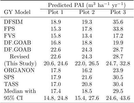
used in the region, which is likely due to the plantation-specific (versus regional) dominant height growth equa-tion used in our study. Our base-projecequa-tion stand BA was 1.9 and 3.7% higher relative to the six model aver-age for plots 1 and 2, respectively, while it was 17.7% lower for plot 3. The source of this difference for plot 3 is unclear; however, two of the growth models, in-cluding ORGANON (Hann et al. 2003), showed similar projections for plot 3 (within 3.5%). With respect to the predicted 20-year periodic annual increment (PAI), which includes uncertainty from both D and H, the re-vised DF.GOAB generally had the highest value (except for plot 3), but it was generally near the median estimate from the other models (Table 5).
Table 5: Derived periodic annual increment (m3 ha−1 yr−1) of various growth and yield (GY) models in the Pacific Northwest for three plots after 20 years of pre-diction. The GY models included DFSIM (Curtis et al. 1981), FPS (Arney 2005), FVS (Crookston and Dixon 2005), DF.GOAB (Weiskittel et al. 2007), SMC-ORGANON (Hann et al. 2003, 2006), SPS (Arney 1985), and TASS (Mitchell 1975) as well as the revised DF.GOAB developed in this analysis, which is presented with a 95% credible interval. For comparison, the over-all median with a 95% confidence interval (CI) was com-puted.
Predicted PAI (m3ha−1yr−1)
GY Model Plot 1 Plot 2 Plot 3
DFSIM 18.9 19.3 35.6
FPS 15.3 17.8 33.8
FVS 15.8 13.4 17.2
DF.GOAB 16.8 18.8 19.9
DF.GOAB 22.6 24.3 28.7
Revised 22.6 24.3 28.7
(This Study) 20.6, 24.6 22.0, 26.5 24.7, 32.8
ORGANON 17.8 16.2 23.9
SPS 17.9 21.6 30.5
TASS 17.0 20.8 30.4
Median with 17.4 18.5 29.5
95% CI 14.8, 24.8 15.4, 27.6 24.6, 43.6
3.2 Error representation
All sources of uncertainty in the system of equations are represented in the Bayesian probabilistic modeling platform. Parameter errors are represented as MVN for each fitted equation, but are considered independent across equations. The database for equation fitting is ex-tensive, so standard errors on parameter estimates are relatively small. However, residual errors and random
effect are relatively large for reference to model perfor-mance (Supplemental Materials S3).
Each iteration of the MCMC represents a full 40-year simulation for all projected trees, and the model took a random MVN draw as the parameter estimates for each iteration. Parameter estimates fully retain the pair-wise linear correlations between parameters, and assign these unique parameter draws to project all individual trees across all years for that single MCMC iteration. Dif-ferent MCMC iterations use various parameter draws from the same MVN distribution. Similarly, random er-ror is partitioned during equation fitting into installation and plot variance components, along with residual error. Each component is considered independent within and between equations (Littell et al. 2006). The Bayesian Network is flexible enough to model this hierarchical er-ror structure, which is necessary given the typical ob-jective of projecting specific field inventoried plots as discrete units rather than as random draws from a pop-ulation. This also allows for the potential to calibrate individual plot- and installation-level random effects. However, without calibration data the installation- and plot-level random effects would be applied as full un-conditional error terms, additive to residual variance. We assessed installation- and plot-level random effects for across equation correlations, but found these to be mainly non-significant, with the largest correlation co-efficient (-0.51) between plot∆H and plot∆D . Residual
errors also had low correlations.
simul-taneously update priors for the plot random effect (i.e., calibration) using the H and HCB data for the specific plot. It should also be noted that log-bias corrections (Flewelling and Pienaar 1981) are not necessary in a Bayesian Network since the back-transformations to the nominal scale are made at the individual tree-level pre-dictions (Stow et al. 2006).
We modeled individual-tree mortality with logistic re-gression. For each projection year the model predicted mortality (yes/no) based on the estimated probability of mortality from the fitted model. Randomly drawn parameter estimates were constant across all projection years within a single MCMC iteration. Predicted mor-tality for each tree in a projection year was taken as a random draw from a Bernoulli distribution with the pa-rameter equal to the projected probability of mortality. Within a single MCMC iteration (i.e., over all yrs), we constrained tree status (live v. dead) to remain dead in future years if a mortality event had occurred. Mortality was the only discrete variable in the model.
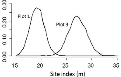
Site index is the only required measure of site quality for the ecological system. Predictions of site index for our illustration plots were relatively imprecise, despite the actual age of the plantations being close to the site index base age of 25 years (Fig. 3). Precision will de-crease for stand ages further from this base, particularly for younger stands. The site index for plot 2 was known exactly (18.4 m at 25 yrs) because the stand was 25 years old. As with all other estimated variables and param-eters, site index is represented in our model as a pos-terior distribution of possible values. This is distinctly different from other forest GY models that apply a point estimate of site index as a known value. Lastly, for two derived variables (MCW and MCA) we took parameter estimates from the literature, but since these were given without standard errors or correlation between parame-ters, these parameters were entered into the model deter-ministically. All derived variables in this model, except some in the starting year, are represented as posterior distributions since they were computed from variables with modeled uncertainty. Certain starting year derived variables, such as BA0 , are based on fully measured
data (and thus assumed to be known with certainty and without any measurement error), which can be an im-portant source of uncertainty in forests (e.g., Gertner 1990).
3.3 Error propagation
Error propagation occurred automatically across com-ponent equations and projection years for all sources and types of errors, including parameter estimation error, residual error, and random effects, as well as uncertainty in stand- and tree-level starting conditions. Plot-level
Figure 3: Derived posterior distributions of site index for plots 1 and 3. Site index for plot 2 was known precisely since it was 25 years old.
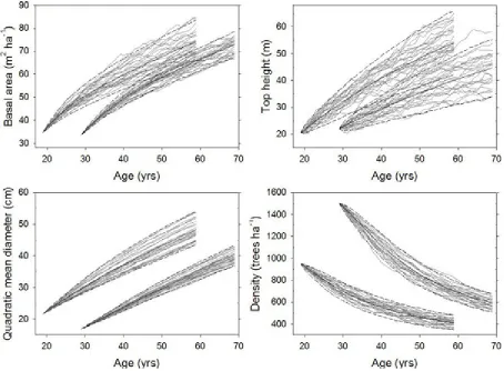
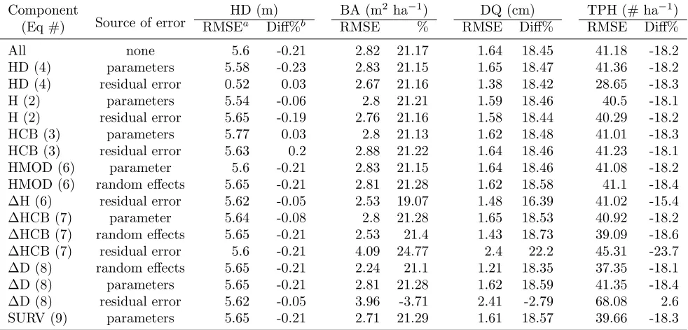
projections showed error propagation across years, with the uncertainty increasing over time (Fig. 4). For illus-tration, stand-level variable projections for Plots 1 and 3 are shown for 25 randomly selected MCMC iterations, plotted relative to the mean and 95% credible interval (Fig. 4). For consistency, the same MCMC iterations were used across all variables. Plot 2 behaved similarly to Plot 1, and is not shown. HD projections [Eq. 4] showed wider credible intervals (Fig. 4), despite precise parameter estimates (Supplemental Materials S3). The primary influence was a relatively large residual error that was additively applied to this non-linear equation in successive projection years. This uncertainty in HD pro-jection resulted in the somewhat wider credible intervals for site index (Fig. 3). Projections for stand-level vari-ables, BA, DQ, and TPH, were somewhat less variable. The 95% credible intervals for BA were approximately symmetric, but increased over the projection period to between 14% and 23% of the mean at 40 years for these plots (Fig. 3). DQ showed similar projection errors av-eraging 18.1% of the mean, while TPH was somewhat less precise, ranging between 24% and 31% of the mean projection.
plot-Figure 4: Base 40-yr projections for Plots 1 and 3 of pure Douglas-fir plantations with initial ages of 29 and 19 yrs, respectively. Plot 2 behaved similarly to Plot 1, so was not shown for clarity. Shown are posterior means (solid heavy line), and 95% credible intervals (dashed lines) for plot-level characteristics. Base projections included all sources of error. Also shown are 25 randomly chosen MCMC iterations from the 4,000 iterations comprising the sampled posterior distributions, keeping the same iterations for all variables.
level variables (e.g., BA and CCF) influence these tree-level projections. However, within a single projection step (i.e., age), the trees were considered independent. Also, Figure 4 illustrates the variability in the mortality projections. As expected from ecological understand-ing, mortality tends to be higher in smaller diameter trees (Fig. 5), but there is also stochastic variability be-tween MCMC iterations. It should also be noted that errors due to parameter and random effects do not av-erage across trees, since these are applied to all trees identically in an MCMC iteration.
3.4 Error budgets
Increasingly wider credible intervals with projection age was simply inherent to the recursive nature of these equations, where prediction error in one year (either tree-level or plot-level variables) were propagated for-ward to the next year, and so on (Fig. 4). Residual
er-ror was considered independent across trees and years, which is an error structure that serves to reduce across-year effects through partial cancellation depending on the random draw. We did not employ an error structure that was constrained across the entire simulation period, or gradually changing (e.g., autoregressive). Thus, the contribution of residual errors to the system-wide pre-diction error was generally higher than when accounting for other sources of error (Table 6).
A full error budget for this forest GY model is be-yond the scope of this paper, since our primary objective was to develop the modeling framework and evaluate the several advantages it can provide. Projection errors for selected plot-level variables are shown in Table 6 for the full base-projection for Plot 1 only, at the 40thprojection
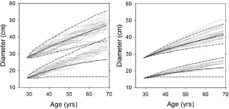
Figure 5: Diameter growth projections for arbitrarily chosen trees 1 and 2 from Plot 1 for the base projection (left) and projection where residual error for diameter growth was set to zero (right). Shown are posterior means (solid heavy line), and 95% credible intervals (dashed lines). Also shown are 25 randomly chosen MCMC iterations from the 4,000 iterations comprising the sampled posterior distributions. Mortality events are shown as an ending line prior to the end of the projection. The credible intervals reflect no diameter growth after a mortality event, so are wider than a dynamic approach that only tracks live trees.
not a simple additive process across all error components (Table 6). HD residual error showed the greatest effect, reducing RMSE from 5.6 to 0.52 m. All HD projections were relatively similar to the deterministic projection, as shown by very small percentage differences. Similarly, H0 and HCB0 estimates were similar to deterministic
estimates, with the RMSE contributing the most to the variability (Table 6), rather than parameter error. How-ever, all of these equations were non-recursive, and were not dynamic across component equations.
Projections of BA and TPH with and without includ-ing residual errors on ∆D illustrate the marked differ-ences between approaches (Fig. 6). The only difference between the two projections is that residual error was set to 0.00001 (i.e., essentially zero). Doing so paradox-ically increased projection error, but also strongly re-duced the projection difference relative to deterministic projections (Table 6). All three plots behaved similarly, and a simple examination of the component equations explains this model behavior.
The individual tree-level ∆D equation shows a highly recursive and dynamic projection function. In simplified terms, diameter growth in each time-step is a function of the starting diameter, other tree-level variables also influenced by D (H and HCB), as well as plot-level de-rived variables involving D, H, and HCB. However, the dominant influence causing the differences shown in Fig-ure 5 is due to a strong interaction between an annual-time step residual error on ∆D and the highly recursive and dynamic form of the ∆D equation. As trees
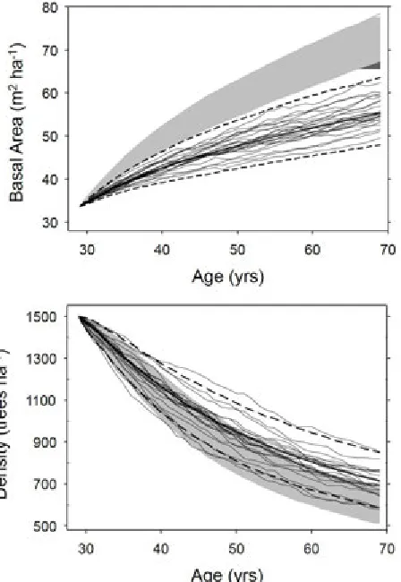
Table 6: Effects of individually removed sources of error for a single component equation, with the component equation and source listed. Results are 40-yr projections for Plot 1 only showing residual error (RMSE), and percentage difference (Diff%) compared to a purely deterministic projection.
Component
Source of error
HD (m) BA (m2ha−1) DQ (cm) TPH (# ha−1)
(Eq #) RMSEa Diff%b RMSE % RMSE Diff% RMSE Diff%
All none 5.6 -0.21 2.82 21.17 1.64 18.45 41.18 -18.2
HD (4) parameters 5.58 -0.23 2.83 21.15 1.65 18.47 41.36 -18.2
HD (4) residual error 0.52 0.03 2.67 21.16 1.38 18.42 28.65 -18.3
H (2) parameters 5.54 -0.06 2.8 21.21 1.59 18.46 40.5 -18.1
H (2) residual error 5.65 -0.19 2.76 21.16 1.58 18.44 40.29 -18.2
HCB (3) parameters 5.77 0.03 2.8 21.13 1.62 18.48 41.01 -18.3
HCB (3) residual error 5.63 0.2 2.88 21.22 1.64 18.46 41.23 -18.1
HMOD (6) parameter 5.6 -0.21 2.83 21.15 1.64 18.46 41.08 -18.2
HMOD (6) random effects 5.65 -0.21 2.81 21.28 1.62 18.58 41.1 -18.4 ∆H (6) residual error 5.62 -0.05 2.53 19.07 1.48 16.39 41.02 -15.4
∆HCB (7) parameter 5.64 -0.08 2.8 21.28 1.65 18.53 40.92 -18.2
∆HCB (7) random effects 5.65 -0.21 2.53 21.4 1.43 18.73 39.09 -18.6
∆HCB (7) residual error 5.6 -0.21 4.09 24.77 2.4 22.2 45.31 -23.7
∆D (8) random effects 5.65 -0.21 2.24 21.1 1.21 18.35 37.35 -18.1
∆D (8) parameters 5.65 -0.21 2.81 21.28 1.62 18.59 41.35 -18.4
∆D (8) residual error 5.62 -0.05 3.96 -3.71 2.41 -2.79 68.08 2.6
SURV (9) parameters 5.65 -0.21 2.71 21.29 1.61 18.57 39.66 -18.3
aRMSE is the standard deviation of the posterior distribution for the 40th projection year.
bDifference relative to a deterministic projection, computed as 100 * (projection mean - deterministic mean) / projection mean,
where the two variables are the means of the posterior distributions. Only one deterministic projection was required.
Random effects and parameter errors did not cause similar differences between our projections and the de-terministic one. These types of errors entered into pro-jections in a fundamentally different way, since they were chosen stochastically once and only once at the begin-ning of each MCMC iterations, and so were fixed across all projection years, whereas residual error was stochas-tically drawn in each projection step (i.e., each projec-tion year).
4
Discussion
This example from a common class of ecological mod-els, namely a recursive system of discrete, difference form equations, was easily and adequately represented within a Bayesian Network. The MCMC approach allowed for mixed discrete and continuous variables, and was suffi-ciently flexible to model a rather complex error struc-ture of our example ecological system. We specifically chose to investigate a Bayesian Network as a modeling platform. The main criteria for this platform were: (1) accurate and tractable projections that include full error propagation, (2) flexible and comprehensive analytic ca-pabilities, (3) allows hierarchical and multi-level model structures, (4) capability for random effects calibration, (5) capability for hypothesis testing and updating
knowl-edge across different system components, simultaneously with different sources of information (i.e., new data), (6) computationally fast, and (7) relatively simple imple-mentation, preferably in a scripting language. Finally, while not one of the formal criteria, the probability inter-pretation of the posterior distributions provides a clear advantage for use within decision support systems (Bor-suk et al. 2004) and is the basis for the natural link be-tween Bayesian approaches and risk assessment (Berger 1985).
Figure 6: Forty year projections for Plot 1, a pure Douglas-fir plantation, where residual error for diame-ter growth was set to zero. Shown are posdiame-terior means (solid heavy line), and 95% credible intervals (dashed lines), as well as 25 randomly chosen MCMC iterations. For reference, 95% credible intervals for the base pro-jection (all sources of error included) are shown as gray outline, which are identical to results from Fig. 4.
The JAGS program was one possible choice, and was shown to be thoroughly adequate. Alternately, for port-ing existport-ing ecological models to a Bayesian Network, be-spoke code could be written for MCMC samplers (Hojs-gaard et al. 2012), and this approach might be preferable for deployment of models past the development stage as it simplifies the amount of recoding of the original model. The primary difficulty with representing a relatively simple Douglas-fir forest GY model as a Bayesian Net-work arose from the highly recursive nature of the equa-tions. The graph moralizing step in constructing the model dependencies is not unduly numerically intensive (Nielsen and Jensen 2009), but tended to cause certain Bayesian software programs to have very long “compile” times, WinBUGS and OpenBUGS in particular. Once the model was compiled in JAGS, running 40,000
iter-ations of the MCMC took 60 to 90 minutes, depending on the number of trees simulated. This compiling is-sue with highly recursive equations is a known problem with these software packages, but was not exhibited for JAGS. Finally, due to the highly connected nature of Bayesian Networks, the models contained an extremely large number of variables (>100,000), with each variable being represented as a posterior distribution of possible values. These included all parameters, random effects, and residual errors, but also each predicted variable for each projection year was considered a unique variable. These included all predicted H0 and HCB0, as well as
separate D, H, HCB and survival projections for each tree over each of the forty years in the projection. De-rived variables at the tree- or plot-level such as CCF and BA had similar representation, each being expressed as posterior distributions for each time step. This highly connected nature of Bayesian Networks adds to their flexibility, but also to their computational load.
4.1 Error budgets
Plot 1 BA was projected to be 72.8±2.82 m2 ha−1 (mean±sd) after 40 years, with 95% CI of 67.3 to 78.5 (Fig. 4). Similar statistically valid errors are available for every projected variable on each plot. Automatic er-ror propagation across the system of equations is a dis-tinct advantage of the Bayesian modeling platform. Few existing ecological models include error estimates with the projections (Larocque et al. 2008), but there are no-table exceptions (e.g., Borsuk et al. 2004, Kershaw et al. 2017). We feel this is a major shortcoming in ecolog-ical modeling, since the usual manner in which model projections are assessed is through estimates of projec-tion error. Without these, it is quite difficult to evalu-ate the adequacy of point estimevalu-ates, or make between-model comparisons. Several methods have been devel-oped to provide error estimates, and these can be clas-sified into Monte Carlo–type simulations or analytical solutions (Lo 2005). Bayesian Networks provide an an-alytical solution (i.e., a full posterior distribution) that is represented through MCMC sampling. Accurate and tractable error estimates are increasingly required for ecological projections, particularly for carbon seques-tration where carbon credits are often tied to an esti-mated lower confidence bound as a conservative measure (Smith and Heath 2001).
for a system of equations generally require tens, if not hundreds of thousands of simulations (O’Neill and Gard-ner 1979). Further, characterizing autocorrelation be-tween parameters and other non-independent variables will necessarily add complexity in specifying the simu-lation space. There are, however, several methods that have been developed to reduce the number of Monte Carlo simulations, notably orthogonal polynomials (e.g., Gertner et al. 1996, Parysow et al. 2000). Results and efficiency of these methods would be comparable to the Bayesian Network approach used in this study, but with their utility restricted to estimating error budgets.
In its simplest form, a Bayesian Network approach to characterize error propagation can be viewed as simply Monte Carlo simulations of a well-conditioned system of equations. That is, if there is no parameter estima-tion through new data (e.g., calibraestima-tion in this context) or other sources of information, then the dependencies of the posterior distributions are explicitly defined as Π(parents). Markov Chain Monte Carlo sequentially samples each variable conditional on the current esti-mate of the other variables, and the dependencies spec-ified in the component equations. The posterior distri-butions (e.g., Fig. 4) are a collection of equally plausible predictions and form statistically valid error estimates. The primary contrast between Bayesian Network and simple Monte Carlo approaches is in the use of stochas-tic draws. The Monte Carlo approach explicitly make a random draw from a known (or presumed known) distri-bution. In cases where parameters are non-independent (e.g., MVN) then random draws for these parameters are conditioned on their covariances. In contrast, ran-dom numbers in MCMC are used to compute a pro-posed step within a random walk (Capp´e and Robert 2000). Assuming the current MCMC iteration is sam-pling from the true posterior distribution for the model, then each subsequent iteration (step) of the MCMC can be used to characterize the posterior distributions. In the simplest Bayesian Network case (i.e., no new infor-mation is provided), when starting value for the chain are chosen with the same error distributions and condi-tional dependencies as in the specified model, then even the first iteration is describing the stationary posterior distribution (Pearl 2000).
A disadvantage to a Bayesian Network approach for error budgets is the inability to provide optimal solu-tions for reducing system error based on a loss func-tion (Lo 2005). This requires an analytical solufunc-tion for error propagation that Gaussian error propagation (Lo 2005) can provide. There are several other analytic ap-proaches to error budgets, including orthogonal polyno-mials (Parysow et al. 2000) and first-order Taylor se-ries approximations of variance (Mowrer 1991). In ad-dition, Bayesian synthesis (Raftery et al. 1995, Green et
al. 2000) is well suited to error characterization in sim-ilarly structured ecological models. Such an approach is ideally suited to characterizing uncertainty where the model parameters are not estimated from data, which is common in mechanistic models (Green et al. 1999). Bayesian synthesis can be used where the mechanistic model structure and parameters are combined with field-collected data from higher-level projections; e.g., BA and TPH at the starting age in our model. The joint pre-model distribution of all input (model parameters) and output (usually field data) are updated using con-temporary Bayesian methods and algorithms to provide a post-model distribution. However, this approach was not applied in this study due to abundant process-level data being available for fitting the component equations.
4.2 Model development and error structure specification
It became quickly evident during model development that incorporating residual errors had a marked influ-ence on projections (Fig. 5). This occurred across all equations that had a recursive component (e.g., ∆D), and it carried forward to derived variables. Using a for-est plantation system, Kangas (1997) showed a similarly increasing pattern of projection error over time from a simple Monte Carlo error propagation approach over 50-year projections. Kangas (1997) also indicated a dif-ference between Monte Carlo means and deterministic projections, although not as large as in our study. Pre-vious studies have also demonstrated differences com-pared to deterministic projections (Dennis et al. 1985; Gertner 1991). In particular, both Mowere (1991) and Kangas (1996) showed clear differences in projections from a structurally similar forest GY model to ours, when residual errors were included. However, while their component equations for ∆D were also recursive, they attributed the resulting difference to non-linear compo-nent equations rather than inherent recursiveness. We submit that the difference is due to both non-linear and recursive equation forms.
dy-namics. There are both positive and negative feedback elements with each of the recursive equations, which act to constrain individual tree- and plot-level growth rates. Other sources causing differences in our model include non-recursive equation components such as an estimated site index. The site index predictions, how-ever, were similar compared to the deterministic predic-tions despite having a strongly non-linear form. This was due to state variables being used in site index com-putations (i.e., top-height and age were field measured without likely significant measurement error). However, site index was still estimated with relatively high error (Fig. 2) and this variable enters into growth increment equations non-linearly, which can therefore result in dif-ferent mean projections from deterministic ones (Table 6). Although these impacts were considerably smaller than the impacts of including residual errors to other component equations, they remain a potentially signifi-cant source of uncertainty.
In this study, we simply noted the marked difference between probabilistic and deterministic growth projec-tions, as have other studies. This is clearly a topic that needs to be resolved, as Bayesian model projections are becoming more common (Clark and Gelfand 2006). The relatively sparse modeling dataset makes it difficult to determine which projection approach is most accurate. We have numerous tree measurements across 167 plots; however, the mean total measurement period for a plot was 12.8 years, with a sd of 4.4. With such short time-series, prediction error is difficult to assess for recur-sive equations. There is considerable additional effort required to fully and accurately characterize the error structures, even for a relatively simple ecological model as this. Nevertheless, we do not view this as a disad-vantage as prediction accuracy does depend on correct model specification, including correct error specification. In addition, model building with a specific aim to reduce projection error will help refine data collection efforts.
4.3 Research integration
The ability of Bayesian Networks to learn and com-municate information by representing the model systems conditional probabilities (Pearl 1988) is, in our opin-ion, the greatest advantage of the probabilistic model-ing framework described in this study. It is also the principal feature that distinguishes Bayesian Networks over alternate modeling platforms. Many of the other attributes, such as error propagation, have clear corol-laries with other analytic techniques; Bayesian Networks provide this collection of advantages in a single platform, with existing MCMC programs greatly simplifying im-plementation. In addition, Bayesian Networks also al-low for very natural and easily understood integration
among discipline-specific models. There has always been a need to integrate research across disciplines, but most modeling efforts remain discipline specific. The need for integrating research across once disparate disciplines is becoming critical as ecological risks associated with cli-mate change become more apparent (Willows and Con-nell 2003).
A direct application of this approach is potentially where site index estimates are unavailable for an estab-lished stand; for example, due to past disease or physical damage to dominant trees so that the dominant trees were not “free to grow” over the entire stand develop-ment, and do not represent site potential. In these cases, the GY models are often applied regardless, but using an approximate estimate of site index or a regional av-erage. However, in the probabilistic model developed in this study, it is entirely possible to substitute field col-lected ∆D or ∆H information to directly estimate the site index, such that information or “message-passing” occurs opposite of the direction of influence (Pearl 1988). For example, a weakly informative uniform distribution for site index could be used as a prior distribution that is then updated with new response data in a conventional Bayesian approach. Multiple types of data can then be used simultaneously to predict site index.
This information passing and learning feature of Bayesian Networks as well as the ability to incorpo-rate new data into model projections forms much of the basis for “model-data fusion” approaches in eco-logical modeling (Fox et al. 2009, Hobbs and Ogle 2011), where model parameters and to some extent model structure are in constant flux as new data be-come available. Model-data fusion approaches are fun-damentally similar to the probabilistic modeling ap-proach taken in our study, although we emphasized model projections and error budgets. The Bayesian Net-work as constructed could immediately be applied to investigate typical model-data fusion questions (Hobbs and Ogle 2011). Data assimilation is another related proach usually implemented around a Kalman filter ap-proach (Houtekamer and Mitchell 1998). The somewhat seamless interplay between contemporary Bayesian pa-rameter estimation and model projection should be em-phasized; both were done simultaneously in this study. The flexible Bayesian parameter estimation approach (Berger 2000, Wikle 2003, Clark and Gelfand 2006) car-ries forward into a similarly flexible modeling platform for projections within a Bayesian Network. Our exam-ple of a relatively comexam-plex system of equations was only one class of ecological model that this framework can express.
political science with ecological or hydrology models. The conditional probability representation of the eco-logical or social processes provides a common language across research domains, while the casual representation allows formal hypothesis testing (in a scientific sense) across research domains. Formal hypothesis testing across research domains is further aided by the prob-abilistic interpretation of the posterior distributions. A flexible probabilistic platform is critical here. Several good examples exist of Bayesian Networks in ecologi-cal modeling; however, most of these are constrained to categorical-only variables (e.g., ARIES model of ecosys-tem services; Villa et al. 2009) or have limited ability to include new data for learning or hypothesis testing (e.g., Marcot et al. 2006). The simplest case of cross-domain hypothesis testing, or learning, comes when projected outcomes of one model are independent variables (i.e., with no parents) in a different model. For more com-plex cross-discipline integration, parameter identifiabil-ity will be challenging, and will need to be addressed through multiple data sources to isolate the processes of interest.
5
Summary
There are many sources of uncertainty present (e.g., systematic error, measurement error, parameter un-certainty) in ecological models (Uusitalo et al. 2015). Bayesian Networks are becoming an important approach for quantifying and understanding this uncertainty (e.g., Uusitalo 2007, Barton et al. 2012). To our knowledge, this is the first development and use of a Bayesian Network to quantify uncertainty in a commonly used individual-tree forest GY modeling framework. The overall projections were consistent with several other re-gional GY models in the Pacific Northwest (e.g., John-son 2005); however, the projections showed a relatively high degree of uncertainty in both estimates of stand-and tree-level attributes even though the framework only addressed uncertainty in the underlying prediction equa-tions and not other additional factors like measurement error. This uncertainty significantly increased with the length of the projection, which is an important finding as most GY projections for both scientific and practical planning purposes are often 50 to 100 years in length. The model forecasts were highly sensitive to error as-sociated with ∆D given that it is the primary variable in this type of modeling framework. This relatively high uncertainty can complicate interpretation of derived GY model outputs, which are generally used for forest finan-cial assessments or planning of specific management ac-tivities (e.g., Weiskittel et al. 2016b). Recognition of this uncertainty and effective incorporation into derived out-puts is necessary for realistic and optimal representation
of the system being forecasted. Overall, the Bayesian probabilistic framework presented here highlights the importance of uncertainty in deterministic modeling and is flexible enough to be adapted to other regions, mod-eling approaches, or ecological systems.
Acknowledgments
Thanks to the University of Washington Stand Man-agement Cooperative and its supporting members for ac-cess to the Douglas-fir plantation data. Development of this manuscript benefited greatly from discussions with Drs. Y. Liang and D. Hann. This study was partially funded by grants to D. Wilson, including the U.S. De-partment of Defense Strategic Environmental Research Development Program (SERDP) project RC-2116, and NSF grant IIA-1301789. Projections were made utiliz-ing the Oklahoma State University high performance computing facility supported through NSF grant OCI-1126330. NSF’s Center for Advanced Forestry Systems (CAFS) and USDA National Institute of Food and Agri-culture, McIntire-Stennis Project Number ME041516 through the Maine Agricultural and Forest Experimen-tal Station partially supported A. Weiskittel’s time on this study. We thank the six anonymous reviewers who provided helpful feedback on an earlier version of this manuscript. M. Fergusson assisted with final editing.
References
An, L. (2012). Modeling human decisions in coupled human and natural systems: Review of agent-based models.Ecological Modelling. 229:25-36.
Arney, J. D. (1985). A modeling strategy for the growth projection of managed stands. Canadian Journal of Forest Research,15(3), 511-518.
Arney, J.D. (2005). Forest Projection System. For-est Biometrics Institute. Portland, OR, USA. http://www.forestbiometrics.com/
Arnold, J. G., & Fohrer, N. (2005). SWAT2000: current capabilities and research opportunities in applied wa-tershed modelling.Hydrological Processes,19(3), 563-572.
Barton, D.N., Kuikka, S., Varis, O., Uusitalo, L., Henriksen, H.J., Borsuk, M., de la Hera, A., Far-mani, R., Johnson, S. & Linnell, J.D. (2012). Bayesian networks in environmental and resource management. Integrated Environmental Assessment and Management,8(3), 418-429.