Electricity Load Demand Forecast using Fast Ensemble-Decomposed Model

(1)

e-ISSN: 2600-7924/penerbit.uthm.edu.my/ojs/index.php/jst

Electricity Load Demand Forecast using Fast Ensemble-Decomposed

Model

Nuramirah Akrom and Zuhaimy Ismail

*

*Department of Mathematical Sciences, Faculty of Sciences, Universiti Teknologi Malaysia, 81310 Skudai, Johor, Malaysia. Received 30 September 2017; accepted 10 June 2018; available online 1 August 2018

1. Introduction

Forecasting electricity load demand has always played a substantial role in generation scheduling, transmission planning, and pricing [1]. The importance of achieving the highest forecast accuracy of electricity load demand is really needed since deregulated companies in the power market depends on it [2].

Basically, forecasting electricity load demand has different forecast horizons. For example, long-term electricity load demand forecasts, ranging from one to ten years ahead of forecast, are necessary for capacity planning of an electricity company, and it also functions

as an economic parameter. Short-term

electricity load demand forecasts, meanwhile, are essential for the day-ahead markets [3].

Long-term patterns of electricity load demand sometimes have irregular components, depending on the consumption of load demand in that year. It is a challenging task to forecast the irregular patterns exhibited in long-term electricity load demand data series [4]. Hence, this creates an opportunity to develop new methods for forecasting long-term electricity load demand and indirectly, this new method can capture the irregular patterns that exist in the electricity load demand data series.

In previous literature, various models have been proposed by researchers in order to model, forecast, and counteract these irregular patterns for long-term electricity load demand

data series. For example, He et al., [5]

proposed four different steps, whereby for each step of the forecasting procedure, they employed four different methods to forecast urban electricity load demand in Tianjin, China. For the first step, they implemented linear regression and moving average method to capture the relationship between variables within the model. Secondly, they applied time

series forecasting methods, which are

Autoregressive Model (AR), Moving Average Model (MA), and Autoregressive Moving Average Model (ARMA), to determine the stationary pattern of the load data. Thirdly, they used grey forecasting model and combined forecasting models of ARIMA and Grey Model to predict the non-linear load

index. Lastly, they utilized Artificial

Intelligent (AI) methods, including Support Vector Machines (SVM), Artificial Neural Networks (ANN), Genetic Algorithm (GA), and Particle Swarm Optimization (PSO), to estimate the sensitivity of the initial value and to perform the long-term load demand

forecast. Trotter et al., [6] presented a

stochastic approach to forecast the climate

Abstract: Electricity load demand forecasting is a complex process since the pattern of electricity load demand data sets varies. To overcome this problem, a fast ensemble-decomposed model was proposed in this work. Firstly, two data sets of electricity load demand, which are electricity consumption and electricity production, were decomposed into two Intrinsic Mode Functions (IMFs). Secondly, the different values of ensemble trials are employed into fast ensemble-decomposed model. Then, the second IMF was used as the intrinsic prediction trend for the actual electricity load demand data sets. Lastly, the second IMF was compared with the actual electricity load demand time series data and the intrinsic prediction trend of the second IMF was forecasted. Simulation results revealed that the FED model better than the ARIMA and ANN methods and different values of ensembles trials do effect forecast accuracy.

Keyword: Fast Ensemble-Decomposed Model (FED); Electricity load demand; Electricity consumption; Electricity production; Forecasting.

(2)

185

change and long-term electricity demand in Brazil. They applied multiple linear regression model to calibrate electricity demand data series and forecasted the data series using the proposed method. Zhao and Guo [7] optimized Grey Modelling (1,1) with Ant Lion Optimizer and Rolling mechanism, namely Rolling-ALO-GM (1,1) model, to predict annual electricity consumption in Shanghai city and China states. The proposed model was compared with Grey Modelling (1, 1), Grey Modelling (1,1) optimized by Particle Swarm Optimization, Grey Modelling (1,1) optimized

by Ant Lion Optimizer, Generalized

Regression Neural Network, Grey Modelling (1,1) with Rolling mechanism, and Grey Modelling (1,1) optimized by Particle Swarm Optimization with Rolling mechanism [7].

Although the development of new

techniques proposed by previous researchers to forecast long-term electricity load demand has been helpful, most of them involve too many steps and procedures, which make them costly and time-consuming to implement.

This study, therefore, develops a new method to forecast long-term electricity load demand using Fast Ensemble-Decomposed (FED) model that involves four simple steps only to model and forecast long-term electricity load demand. In addition, there is no need to combine or hybrid the FED method with other methods. Firstly, the original data sets are decomposed into two Intrinsic Mode Functions (IMFs) using FED algorithm. Secondly, the different values of ensemble trials are employed into fast ensemble-decomposed model Thirdly, the second IMF is used as the intrinsic prediction trend for the actual data series. Lastly, the intrinsic prediction trend is forecast.

To demonstrate the effectiveness of the FED model, two data sets were deployed in this study, which are the annual electricity consumption and electricity production in Malaysia. The proposed FED model was compared with ARIMA and ANN models, where these two models also acted as the benchmark methods. This study also aiming to investigate whether the different values ensemble trials do affect the forecast accuracy or not.

The rest of the paper is organized as follows. Section 2 describes the data pattern of the annual electricity consumption and electricity production in Malaysia. Section 3

presents the methods and forecast accuracy measurement used in this study, which are ARIMA, ANN, FED, and Mean Absolute

Percentage Error (MAPE). Section 4

demonstrates the procedure in modelling and forecasting long-term electricity load demand using the three different methods. Section 5 discusses the experimental results and lastly, the conclusion is drawn at the end of this paper.

2. Data Sets.

The electricity load demand data sets cover

the annual electricity production and

electricity consumption in Malaysia, from the

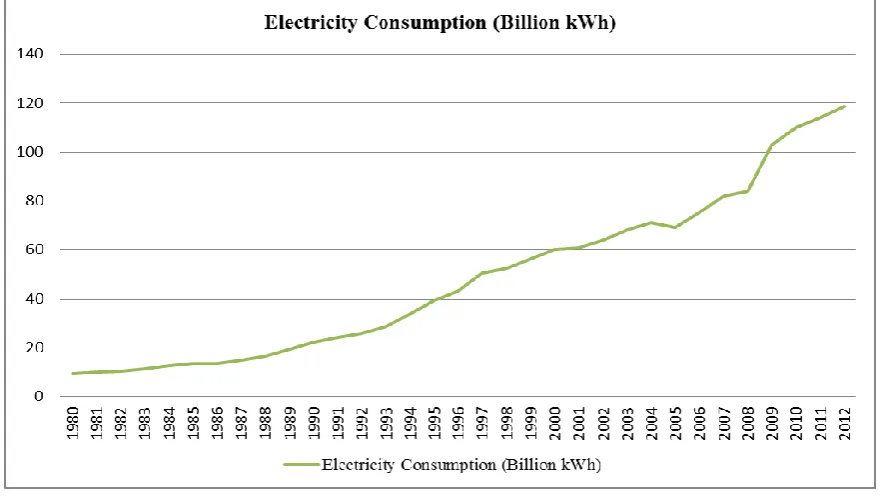
start of 1980 to the end of 2012. Both data gave 64 observations and were measured in kilo-watt per hour (kWh). The data are gathered from Statistical Department of Malaysia. The time series plots for both data are visualized in Fig. 1 and Fig. 2.

Both plots on the electricity load production and consumption showed an exponential pattern, whereby they gradually increased starting from the year 1993 for both data sets. Between 2005 and 2012, the pattern of electricity production and electricity consumption showed a superposition of several distinct frequencies. There were also several fluctuation patterns for the past 7

years, where some complexities and

uncertainties were exhibited in the data series.

3. Methodology 3.1 ARIMA Model.

Generally, the ARIMA ( , , )p d q model is

expressed as [8]:

( )(1

)

d

( )

p

B

y

t

c

q

B

t





 





(1)

where

1

1 P,

p B pB



 



 



1

( ) 1 q

q B B qB



 



 



and

c

is the constant value,

y

_t and



_t are the

actual time series data and error term in a

period of t,

B

is the backshift operator,

d

is

the degree of differencing, and



_pand



_qare

the autoregressive and moving average

(3)

186 Fig. 1 Time series plot for electricity production (billion kWh) from 1980 to 2012

Fig. 2 Time series plot for electricity consumption (billion kWh) from 1980 to 2012

3.2 ANN Model.

Mathematically, a nonlinear ANN model is bounded and parameterized in the form of [9]:

1 2 1 2

( , , , _n; , , , _p) ( ; )

O f x x x

 



 f x



(2)

where

o

is the output layer of the neuron,

f

(.)

is a

nonlinear activation function,

1 2

( ,

,

_n

)

x



x x

x

is the entry vector

variables into the neuron and

1 2

( ,

,

_n

)

(4)

187 3.3 FED Model.

FED was firstly popularized by Wang et

al., [10] is a renovated Ensemble Empirical

Mode Decomposition (EEMD) model,

developed by Wu and Huang in 2009 [11]. Basically, the FED algorithm can decompose any complex time series data into Intrinsic Mode Function (IMF); and the decomposition process as follows [10-12]:

Step 1: Obtain time series signal

Y t

( )

by

adding white noise

n t

_

( )

to the targeted time

series signal,

y t

( ),

( )

Y t



y t



n t

_ (3)

where



1, 2, 3, ,n is the number of

ensemble trials to add into the noise series

inside the original signal, y t( ).

Step 2: Connect all upper, e_up₁ and lower,

1

low

e

envelopes of Y t( )by utilizing cubic

spline interpolations.

Step 3: Calculate the average envelope values between the upper and lower envelop:

1 1 1

( )

2

up low

e

t

e

t

m t





(4)

Step 3: Obtain the difference between Y t( )

and

m t

₁

( )

:

D t

₁

( )



Y t

( )



m t

₁

( )

(5)

Step 4: Judge whether or not

D t

₁

( )

satisfies

IMFs condition, If it does, it is accounted as IMF1, otherwise, it is examined as the original sequence, and the steps 1 to 3 are repeated into

k

rounds.

The IMFs condition have the following properties:

a) In the whole data series, the number of

zero points and the number of extreme points are equal or differ at most by one.

b) The mean vales of the upper and lower

envelopes at any point must be zero.

In this study, the number of IMFs was simply set as 2, since we only needed 2 IMFs

and the ensemble trials are group into [0,100] intervals with 10 increments.

3.4 Forecast Accuracy Measurement.

To evaluate the forecast accuracy of these three methods, Mean Absolute Percentage Error (MAPE) was used as the forecasting accuracy measurement. The equation for calculating MAPE is as follows:

1

ˆ 1

| | 100

N

t t

A F

MAPE X

N  A







(6)

where

A

_t and Fˆ_t are the actual and forecasted

data, and

N

is the number of observations in

the data series.

4. ARIMA, ANN and FED Modelling and Discussions.

To model the annual electricity production and electricity consumption data series using ARIMA model, the procedure as proposed by Box et al., [8] is as follows.Firstly, both data

were differenced

(

d



1)

to transform the

non-stationary series into stationary series. Secondly, the Autocorrelation Function (ACF) and Partial Autocorrelation Function (PACF)

were used to determine the model orders of

p

and

q

. Then, for estimating the parameters of

autoregressive and moving average

parameters,



and



, the Minitab 16 software

was used. After several trials-and-errors, ARIMA (1,1,0) was chosen as the best ARIMA model for both data.

For ANN modelling, a three Multilayer Preceptor (MLP) feed-forward network was developed for predicting the electricity load demand. We also carried out trial-and-error process in calculating the best ANN architecture for both electricity load demand time series data. After several tries, [2-5-1] ANN architecture was chosen for electricity production time series data while [2-4-1] model was the chosen one for electricity consumption.

To model electricity load demand data using FED model, a Matlab 2017 code was built using the FED algorithm to decompose

the original electricity production and

(5)

188

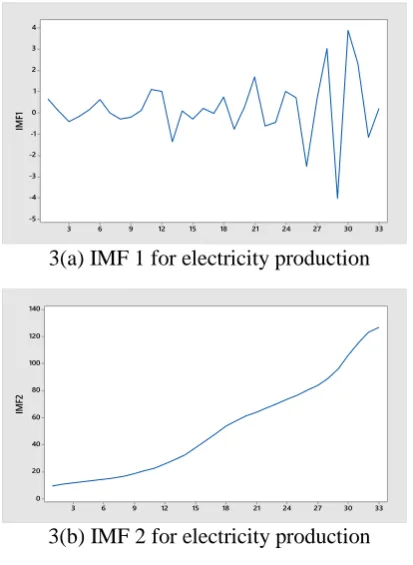
and Fig. 4 depict the IMFs of electricity production and electricity consumption data series.

3(a) IMF 1 for electricity production

3(b) IMF 2 for electricity production

Fig. 3 The IMFs for electricity production

4(a) IMF 1 for electricity consumption

4(b) IMF 2 for electricity consumption

Fig. 4 The IMFs for electricity consumption

From Fig. 3 and Fig. 4, the first IMF of both electricity load demand data series showed high frequencies and high spikes, and although at the beginning the frequency was not too high, starting from the 21st to 32nd frequencies, the spikes were clearly visible. These high spikes depict the start of high demands for electricity from the year 2005 to 2012. As for the second IMF, both data showed an exponential prediction trend of the

electricity production and electricity

consumption time series data. The second IMF was used to forecast the annual electricity load demand.

This study also is used to examine the effect of different number ensemble trials to the forecast accuracy. Table 1 depicts the results of MAPE with different values of ensemble trials.

Table 1 The effect of forecasting performance with different values of ensemble trials

Number of Ensemble Trials Data Electricity Production (MAPE %) Electricity consumption (MAPE %)

0-10 1.7402 1.9830

10-20 1.6687 2.7208

20-30 1.8456 2.0607

30-40 1.6389 1.8374

40-50 1.7900 1.7553

50-60 1.5718 1.9021

60-70 1.5797 1.7473

70-80 1.7458 2.0823

80-90 1.7285 1.8969

90-100 1.7731 1.8760

From Table 1, the best forecast

performances for electricity production is 1.5718% which only needs 50-60 ensemble trials while electricity consumption data need 60-70 ensemble trials for 1.7473 % of MAPE.

Huang et al., [13] proposed the maximum

number of ensemble trials for FED model is 100. Too many ensemble trials may lead to instable extrema distribution and indirectly effect the forecast accuracy.

5. Forecasting Results and Discussions.

To compare the forecasting performance of the three methods, both electricity load demand data had been divided into two groups, which are in-sample data and

(6)

189

sample data. For in-sample data, it consisted of 25 observations from 1980 to 2005 and for out-sample data, it consisted of 8 observations from 2006 to 2012. Table 2 shows the forecasting performance of the three models for electricity production and electricity consumption time series data. For FED model, the best number ensemble trials with the best MAPE are choose to demonstrates the effectiveness of this model

Table 2 Forecasting performance of ARIMA, ANN, and FED models

Electricity Production

Models MAPE (%)

In-sample Out-sample

ARIMA 4.2640 4.7750

ANN 4.0822 8.3248

FED 1.3097 2.3912

Electricity Consumption

Models MAPE (%)

In-sample Out-sample

ARIMA 4.6755 5.4638

ANN 4.0583 4.6337

FED 1.3751 2.9108

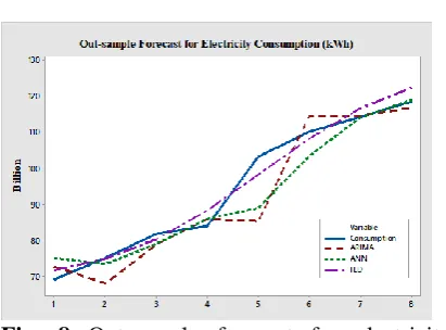
Table 2 shows that the FED model gave the highest forecast accuracy for both types of electricity load demand data as compared to ARIMA and ANN models. This was because the smooth exponential prediction trend of the second IMF in the FED algorithm gave a prediction trend that was closer to the actual electricity load demand data. The worst forecast was by the ANN model, as a result of using hyperbolic tangent sigmoid function in the input neuron and linear sigmoid function in the output neuron. After several trials-and-errors, these two sigmoid functions gave the lowest MAPE. At the end of the 8 observations of the electricity production and electricity consumption, the prediction values using ANN were far from that of the actual values. For ARIMA model, the beginning of the prediction curve followed the actual electricity load demand time series data closely, but towards the end of the prediction curve there were high spikes that gave prediction values that were far from the actual values. Fig. 5 to Fig. 8 illustrate the in-sample and out-sample forecasts using these three models.

Fig. 5 In-sample forecast for electricity production (kWh)

Fig. 6 Out-sample forecast for electricity production (kWh)

Fig. 7 In-sample forecast for electricity consumption (kWh)

(7)

190 6. Conclusion

A new technique for forecasting annual electricity load demand using FED model was proposed in this study. Two types of electricity load demand data were used to demonstrate the effectiveness of the FED model, which are annual electricity production and electricity consumption data series. The FED model was compared with ARIMA and ANN models. The empirical results showed the robustness of the FED model, which gave a range of MAPE between 1% and 2% only, as compared to ARIMA and ANN models which give a range of MAPE between 4% and 5%.

The different values of ensemble trials

do effect the forecast performances. The

number of ensemble trials in FED model

need to clearly investigates and clarify

since its

determine the correctness

distribution of extremum.

Acknowledgement

This study is supported by UTM Tier 1 Grant (11H89) and MyBrain 15.

References

[1] Yukseltan, E., Yucekaya, A., and Bilge, A.

H. (2017). “Forecasting Electricity

Demand for Turkey: Modelling Periodic Variations and Demand Segregation” in

Applied Energy, Vol. 193. pp. 287-296.

[2] Laouafi, A., Mordjaoui, M., Haddad, S.,

Boukelia, T. E. and Ganouche, A. (2017). “Online Electricity Demand Forecasting

Based on an Effective Forecast

Combination Methodology” in Electric

Power System Research, Vol. 148, pp. 35-47.

[3] Koprinska, I., Rana, M. and Agelidis, V.

G. (2015). “Correlation and Instance Based Feature Selection for Electricity

Load Forecasting” in Knowledge-based

Systems, Vol. 82, pp. 29-40.

[4] Shao, Z., Fu, C., Yang, S-L. and Zhou,

K-L. (2017). “A Review of the

Decomposition Methodology for

Extracting and Identifying the Fluctuation Characteristics in Electricity Demand

Forecasting” in Renewable and

Sustainable Energy Reviews, Vol. 75. pp. 123-136.

[5] He, Y., Jiao, J., Chen, Q., Ge, S., Chang,

Y. and Xu, Y. (2017). “Urban Long Term Electricity Demand Forecast Method Based on System Dynamics of the New Economic Normal: The Case of Tianjin” in Energy, Vol. 133. pp. 9-22.

[6] Trotter, I. M., Bolkesjo, T. F., Feres, J. G.

and Hollanda, L. (2016). “Climate Change and Electricity Demand in Brazil: A

Stochastic Approach” in Energy, Vol. 102.

pp. 596-604.

[7] Zhao, H. and Guo, S. (2016). “An

Optimized Grey Model for Annual Power

Load Forecasting” in Energy, Vol. 107.

pp. 272-286.

[8] Box, G. E. P., G. M. Jenkins, G. M., and

Reinsel, G. C. (2008). Time Series

Analysis: Forecasting and Control, 4th Edition. John Wiley and Sons, Inc, New Jersey.

[9] Haykin, S. (2009). Neural Networks and

Learning Machines. Third Edition. Pearson Education, New Jersey.

[10] Wang, Y-H., Yeh, C-H., Young, H-W.

V., Hu, K. and Lo, M-T. (2014). “On the

Computational Complexity of the

Empirical Mode Decomposition

Algorithm” in Physica A: Statistical

Mechanics and Its Applications. Vol. 400. pp. 159-167.

[11] Wu, Z. and Huang, N. E. (2009).

“Ensemble Empirical Mode

Decomposition: A Noise-Assisted Data

Analysis Method.” Advances in Adaptive

Data Analysis. Vol. 1(1). pp. 1-41

[12] Liu, H., Tian, H., Liang, X., and Y. Li,

(2015). “New Wind Speed Forecasting

Approaches using Fast Ensemble

Empirical Mode Decomposition, Genetic Algorithm, Mind Evolutionary Algorithm and Artificial Neural Networks” in

Renewable Energy, Vol. 83. pp. 1066-1075.

[13] Huang, N. E., Shen, Z., Long, S. R., Long,

S. R., Wu, M. C., Shih, H. H., Zheng, Q., Yen, N-C., Tung, C. C., and Liu, H. H.

(1998). “The empirical mode

decomposition and the Hilbert spectrum for nonlinear and non-stationary time

series analysis” in Proceedings of the