An Improved Volumetric Estimation Using Polynomial Regression

An Improved Volumetric Estimation

Using Polynomial Regression

Noraini Abdullah, Amran Ahmed and Zainodin Hj. Jubok School of Science & Technology, Universiti Malaysia Sabah,

Jalan UMS, 88400 Kota Kinabalu, Sabah, Malaysia

Corresponding emails: [email protected], [email protected], [email protected]

Abstract

The polynomial regression (PR) technique is used to estimate the parameters of the dependent variable having a polynomial relationship with the independent variable. Normality and non-linearity exhibit polynomial characterization of power terms greater than 2. Polynomial Regression models (PRM) with the auxiliary variables are considered up to their third order interactions. Preliminary, multicollinearity between the independent variables is minimized and statistical tests involving the Global, Correlation Coefficient, Wald, and Goodness-of-Fit tests, are carried out to select significant variables with their possible interactions. Comparisons between the polynomial regression models (PRM) are made using the eight selection criteria (8SC). The best regression model is identified based on the minimum value of the eight selection criteria (8SC). The use of an appropriate transformation will increase in the degree of a statistically valid polynomial, hence, providing a better estimation for the model.

1. Accordi stronges needed forest st estimatio Stem Bi The vari diameter of log (A respectiv and At (a

then be c Area =л =лD

The volu Figure 1 biomass Newton The obje polynom 2. 2.1 In regre normalit method and the n>50) an 5% whic the depe transform or drivin paper w and opti simulati the type INTRODUC ng to Becht st predictor i for model e and developm on using mu iomass Volu

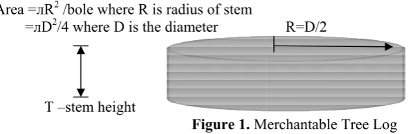
iables consid r at the midd A) is given b ve sections o at the top). S calculated as лR2 _{/bole whe}

D2/4 where D

T –stem heig

ume of the m 1 above. In s is then calcu

’s Formula (

ective of this mial regressio

METHODO Data Prepa ession analys ty test is ini as supportin test statistic nd Shapiro W ch is the stan

The type of endent varia mation value ng down the will focus on imizes the r ons and opti Transformat s of transform

CTION old (2004), in all models enhancement

ment, Norain ltiple regress umetric Equ

dered during dle (Dm), diam

by formula л of the log, th Since diamet s: Ab= лDb 2/4

ere R is radiu D is the diam

ght F merchantable

this paper, ulated using Fuwape et a

s study is to c ons (PR) tech

OLOGY aration and P

sis, normality itially carrie ng evidence c of the varia

Wilk (for n< ndard percent transformati able over the es are taken e ladder will the searchin range of tran

mization. tion will inv

mation need

the stem (or s of tree esti . While Has ni et al.(2008 sion models. uation

g field data c meter at the лR2_{, where R}

he area will t ter is twice t 4, Am= лDm

us of stem meter

Figure 1. M e log will be

based on th the Newton’ l., 2001):

compare mod hnique with

P-value Met y and linear ed out nume

(Ashish & M able is given <50). The con tage of the n ion will be d e independen

to form the l depend on ng efforts for nsformation volve: i) iden

ed, and iii) e

r bole) diam imations, an senaeur (200

8) had presen

collection of top (Dt), and

R is the radiu then be know

he radius, th

2_{/4 and A} t= л

R=D/2

Merchantable e the stem h hese mensur ’s formula as

6

Nw

T

V 

dels based on significant a

thod for Nor relationship erically (Coa Muni, 1990). n by the stat nfidence lev normality test done on any

nt variable. characteriza the concavi r the best tra needed. The ntifying the t exercise the p

meter was sta d for some s 06) had used nted for tree

f 130 trees a d the stem he us of the tree wn as Ab (at

he correspond лDt 2/4 respe

Tree Log height multip

ation variab s in (1).

4 (

6 Ab Am T



n the Newton ttribution to

rmality p of data is o akes & Steed . Normality tistic value o vel is set at 9

t.

data sets by For normali ation of the p ity or conve ansformation ese have als types of curv procedures fo

atistically sig species a qu d modelling stem bioma

are diameter eight (T). The

stem or bole the base), A ding cross-se ctively.

plied by the a les, the volu

)

t

A 

n’s Formula the power te

of prime imp d, 2007), w

tests are car of Kolmogor 95% with sig first plotting ity and linea polynomial te xity of the s ns applicable

o become a vilinear data for Ladder-Po

gnificant and uadratic term

to predict fu ass prediction

at the base e cylindrical e. Hence, at Am (at the mid

ectional area

area as show ume of the

using the erms.

portance. He ith the grap rried out in S

rov-Smirnov gnificance of g a scatter pl arity, approp erms. Drivin scatter plot. e to the data a part of mo

a, ii) determi ower or Box

d the m was future n and

(Db),

transformations. The ladder transformation procedure uses the data sets the power of the origin is employed, which is given by: (Devore & Peck, 1993)

Transform value = (Original Value) power ₍₂₎

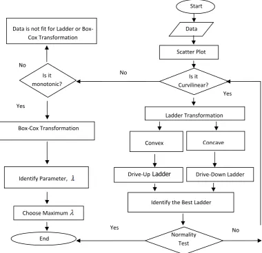
Using the p-value from the F-statistics, data with p-value>0.05are considered as normal. Several iterations are executed so to determine the best transformation required for normality. Figure 2 depicts the flowchart on the data transformation procedures executed on non-normal or nonlinear data before any model building can be developed.

Figure 2. Flow Chart on the Procedures of Data Transformations

2.2 Modelling and Model-Building Approach

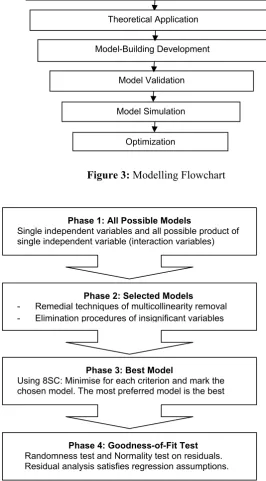
Figure 3 depicts the modelling flowchart. Preliminary with the conceptual development of the importance of modelling, its estimations, and contributions to the real world problems, mathematical theories are applied for model building.

Identify Parameter,    

Concave

Identify the Best Ladder  Start 

     Scatter Plot

Normality  Test 

Data 

Is it  Curvilinear? Is it 

monotonic? 

Ladder Transformation 

Box‐Cox Transformation  Data is not fit for Ladder or Box‐

Cox Transformation 

Drive‐Up Ladder

Choose Maximum   

Drive‐Down Ladder 

End 

No No 

Yes 

Yes 

Convex

Figure 3: Modelling Flowchart

Figure 4. The Four Phases in Model-Building Development

Figure 4 shows the four phases of the Model-building development. Model-building techniques are exemplified and validated through tests and hypotheses. Model’s validation is enhanced by simulation and optimization of values, expected to be characterized as optimal values. In this paper, the phases in model development will not be illustrated since the elimination procedures had been shown by Noraini et al., (2008) and the multicollinearity removal techniques (Noraini et al., 2010(a)).

Phase 1: All Possible Models

Single independent variables and all possible product of single independent variable (interaction variables)

  Phase 2: Selected Models

- Remedial techniques of multicollinearity removal - Elimination procedures of insignificant variables

  Phase 3: Best Model

Using 8SC: Minimise for each criterion and mark the chosen model. The most preferred model is the best

Phase 4: Goodness-of-Fit Test

Randomness test and Normality test on residuals. Residual analysis satisfies regression assumptions.

Conceptual Development

Theoretical Application

Model Validation

Model Simulation Model-Building Development

2.3 Polynomial Regression Models (PRM)

Phase 1 of Model-building in Figure 4, consists of the all possible models which are made up of variables that have been prepared after undergoing the data preparation procedures of Figure 2. For simplicity, these variables are then known as the defined transformed variables.

The PR models are made of a dependent variable, V, the stem volume and single independent variables, taken from field data mensuration. The model-building is developed based on the method of multiple regressions, a statistical method of more than two independent variables as in (3),

Y

_i





₀





₁

X

_1i





₂

X

_2i



...





_k

X

_ki





_i (3) , where i=1, 2, …, n; Yi is the dependent variable; X1i, X2i, …, Xki are the independent variables;

s

'

i



are the regression coefficients with k parameters and εi are the residuals. As with

polynomials of the order 2 (parabolic curve with quadratic terms), the model equation can be written as:

Y_i 



₀ 



₁X_1i 



₁₁X_1i2 ...



_kX_ki 



_kkX_ki2 



_i (4) Based on say four single independent variables, the number of models then is 32 models (as shown in Table 1).

Table 1: Total Number of Possible Models

Number of Variables

Single Independent Variables

Order of Interactions Total number of models 1st 2nd 3rd

1 4 - - - 4

2 6 6 - - 12

3 4 4 4 - 12

4 1 1 1 1 4

Total 15 11 5 1 32

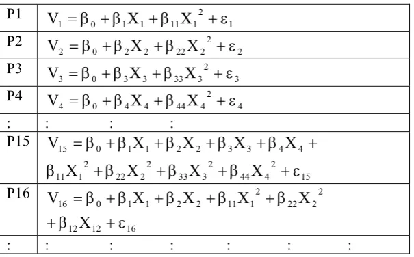
Examples of possible PRM’s are shown in Table 2 whereby models from P1-P15 are without interactions, P16-P26 (1st order interactions), P27-P31 (2nd order interactions) and P32 (3rd order interactions). The all possible PR models are listed as in the Appendix.

Table 2: All Possible Models of Four single independent Variables.

P1

1 2 1 11 1 1 0

1 X X

V    

P2

2 2 2 22 2 2 0

2 X X

V    

P3

3 2 3 33 3 3 0

3 X X

V    

P4

4 2 4 44 4 4 0

4 X X

V    

: : : : P15

15 2 4 44 2 3 33 2 2 22 2 1 11

4 4 3 3 2 2 1 1 0 15

X X

X X

X X

X X

V

  

 

 

 

          

P16

16 12 12

2 2 22 2 1 11 2 2 1 1 0 16

X

X X

X X

V

  



  

      

P27

27 123 123 23 23

13 13 12 12 2 3 33 2 2 22

2 1 11 3 3 2 2 1 1 0 27

X X

X X

X X

X X

X X

V

  

 

 

 

 

 



         

: : : : : : : P32

32 1234 1234 123

123 34 34

12 12 2

1 11 1

1 0 37

X ...

X X

... X ...

X ...

X V

  

  

 



 

  

     

One of the possible models with different variables’ attributes is given by model P27:

27 123 123 23 23 13 13 12 12

2 3 33 2 2 22 2 1 11 3 3 2 2 1 1 0 27

X

β

X

β

X

β

X

β

X

β

X

β

X

β

X

β

X

β

X

β β

V

  

 



 

 

 



(5)

, with X1, X2, and X3 as the single independent variables, X12, X13 and X23 as the 1st order

interactions, X123 is the 2nd order interaction, and X12, X22 and X32 as the polynomial term of power

2 ( or also known as the quadratic terms).

The models can then be written in a general form as:

V

_PR



Ω

₀



Ω

₁

W

₁



Ω

₂

W

₂



...



Ω

_k

W

k



u

, (6) , where VPR is the volume, ‘W’ is an independent variable which represents one of these types of

variables, namely, single independent, interactive, generated, transformed, quadratic terms or even dummy variables, Ω’s are the newly defined regression coefficients, and ‘u’ as the error terms for each respective transformed model. The number of models will depend on the number of single independent variables, given by the formula

(

)

1

j q

j q

_C

j





where ‘q’ is the number of single independent variables.

2.4 Multicollinearity Removal and Insignificant Variable Elimination

Multicollinearity is a phenomenon where there exists very strong linear or perfect relationships between the independent variables (Gujarati, 2006), and collinearity between the variables can be identified by examining the values of the correlation matrix of the independent variables. High correlation coefficients of absolute values in the range of 0.75≥|r|≥0.95 are considered to exhibit multicollinearity effects. These multicollinearity source variables have to be dealt with first before modelling can be done, as indicated in Phase 2 of model development in Figure 3. The elimination of insignificant variables from the models is carried out using the backward elimination method. Illustrations of the backward elimination method had also been shown by Noraini et al. (2008). In this paper, multicollinearity source variables with high correlation coefficient of absolute values greater than 0.95 (|r|≥0.95) are removed. The Case Types for multicollinearity removal procedures had also been illustrated by Noraini et al. (2010)(b).

2.5 Best Model Selection and Goodness-of-Fit Tests

Table 3. Eight Selection Criteria (8SC) for Best Model Identification

AIC (Akaike, 1974) (2(k 1)/n)

e n

SSE 

    

 RICE (Rice, 1984) 1

) 1 ( 2 1

   _

 

   

       

n k

n SSE

FPE (Akaike,1970)

) 1 (

) 1 (

 

 

     

k n

k n

n

SSE SCHWARZ (Schwarz,

1978) n k n

n

SSE _{( 1)/}

     

GCV (Golub etal., 1979)

2 1 1

  

  



           

n k n

SSE SGMASQ

(Ramanathan, 2002)

1 ) 1 ( 1

  

  

      

n k n

SSE

HQ (Hannan &

Quinn, 1979) n k n

n

SSE _{2( 1)/}

ln 

    

 SHIBATA (Shibata,

1981) _ SSE_n _ n  2(_nk 1)

The best model will undergo the goodness-of-fit tests of Phase 4 in Figure 4, which comprises of the normality and randomness tests on the models’ residuals. Without violating the assumptions in regression analysis, further simulations of the best model will provide a better prediction for future forest planning strategy and management.

3. MODELING RESULTS AND ANALYSES 3.1 Normality and Descriptive Statistics

The data variables are measured from 130 trees non-destructively, as defined in Table 3. Normality tests are done and transformations are carried out using Ladder-Power on the non-normal data. Table 4 depicted the defined variables, before and after transformations.

Table 4. Definition of Variables Before and After Transformation Variable Definition Transformation Transformed Variables VNw Stem Volume.(m3):

Nw-Newton

VNw V

Dt Diameter at top of trunk Dt3.7 X1

Dm Diameter at middle of trunk Dm4.5 X2

Db Diameter at the base of trunk Db/T X3

T Tree height (m) T X4

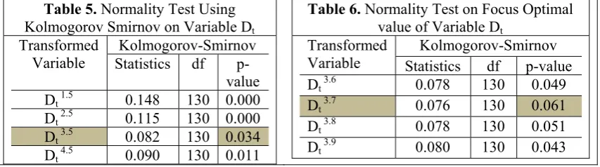
From Table 5, the p-values of variable Dt increase in the variable power range of 1.5–3.5,

before decreases to the value of 4.5. The optimal (highest) p-value is 0.034, and the variable power is thus focused at 3.5.

Table 5. Normality Test Using Kolmogorov Smirnov on Variable Dt

Transformed Variable

Kolmogorov-Smirnov Statistics df

p-value

Dt 1.5 0.148 130 0.000

Dt 2.5 0.115 130 0.000

Dt 3.5 0.082 130 0.034

Dt 4.5 0.090 130 0.011

Table 6. Normality Test on Focus Optimal value of Variable Dt

Transformed Variable

Kolmogorov-Smirnov Statistics df p-value

Dt 3.6 0.078 130 0.049

Dt 3.7 0.076 130 0.061

Dt 3.8 0.078 130 0.051

Dt 3.9 0.080 130 0.043

Transformation power range is then chosen between 3.5- 4.5. Referring to Table 6, variable Dt has reached the optimal normality value of 0.061(highest) at the transformation value

of 3.7. The second decimal digit will lie between 3.7-3.8. Similar procedures are executed on the other variable, Dm, and a generated variable, Db/Th, has been created for normality. Table 7 below

variables have turned to normal since the significant p-value are more than 0.05. The data sets can then be used for further regression analysis.

Table 7. Descriptive Statistics of Transformed Variables

Defined Variables Transformed Variables

V X1 X2 X3 X4

Mean 0.9215 0.1360 0.1081 0.1070 6.1303

Variance 0.133 0.005 0.004 0.000 0.896

Std. Deviation 0.3643 0.0713 0.0628 0.0144 0.9466

Minimum 0.18 0.01 0.00 0.07 3.78

Maximum 1.96 0.40 0.33 0.15 8.23

Skewness -0.020 0.331 0.332 0.624 -0.257

Kurtosis -0.147 0.602 0.158 0.905 -0.378

Kolmogorov-Smirnov 0.068 0.076 0.060 0.065 0.043

Kolmogorov-Smirnov (sig. p-value) 0.200 0.061 0.200 0.200 0.200 Standard error (s.e.) of Skewness is 0.212. Standard error (s.e.) of kurtosis is 0.422.

3.2 Multicollinearity Removal and Backward Elimination Method

In Phase 2 of model-building, multicollinearity source variables with high correlation coefficient of absolute values greater than 0.95 (|r|≥0.95) are thus removed. The Case Types for multicollinearity removal procedures had been illustrated by Noraini et al. (2010)(b).The elimination of insignificant variables from the models is carried out using the backward elimination method.

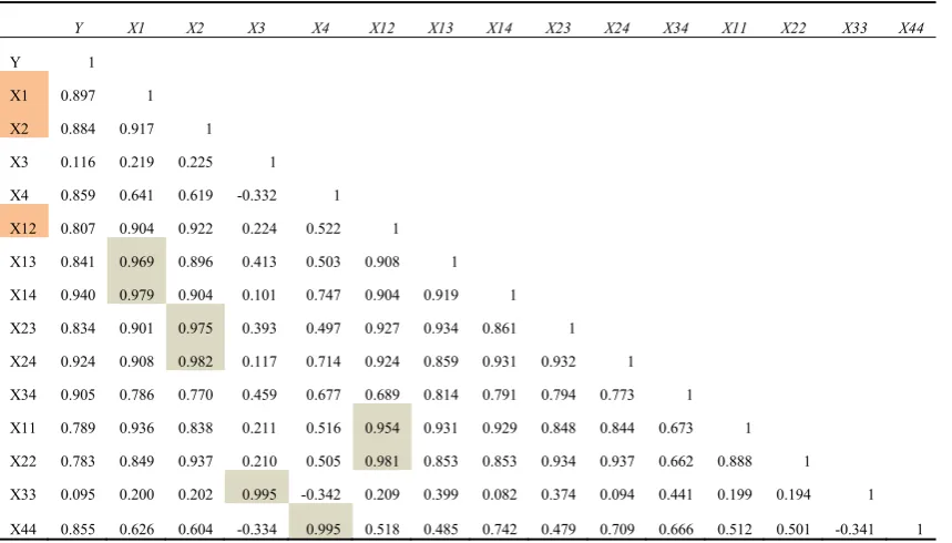
These procedures employed in Phase 2 will not be dealt with in detail, but then suffices to include the coefficient correlation matrix of the best model before and after multicollinearity removal and elimination of insignificant variables being carried out (Table 8, Table 9 and Table 10) respectively. The highlighted values in Table 8 indicate examples of high correlation values exhibiting multicollinearity effects of the independent variables (X1, X2, X12) which then result in the first multicollinearity removal of variable X12.

Table 8: Correlation Coefficient Matrix of Model P26.0

Y X1 X2 X3 X4 X12 X13 X14 X23 X24 X34 X11 X22 X33 X44

Y 1

X1 0.897 1

X2 0.884 0.917 1

X3 0.116 0.219 0.225 1

X4 0.859 0.641 0.619 -0.332 1

X12 0.807 0.904 0.922 0.224 0.522 1

X13 0.841 0.969 0.896 0.413 0.503 0.908 1

X14 0.940 0.979 0.904 0.101 0.747 0.904 0.919 1

X23 0.834 0.901 0.975 0.393 0.497 0.927 0.934 0.861 1

X24 0.924 0.908 0.982 0.117 0.714 0.924 0.859 0.931 0.932 1

X34 0.905 0.786 0.770 0.459 0.677 0.689 0.814 0.791 0.794 0.773 1

X11 0.789 0.936 0.838 0.211 0.516 0.954 0.931 0.929 0.848 0.844 0.673 1

X22 0.783 0.849 0.937 0.210 0.505 0.981 0.853 0.853 0.934 0.937 0.662 0.888 1

X33 0.095 0.200 0.202 0.995 -0.342 0.209 0.399 0.082 0.374 0.094 0.441 0.199 0.194 1

Subsequent five multicollinearity source variables (X1, X2, X12, X11,X44) are being removed have resulted in the correlation coefficient matrix of model P26.5.0 as shown in Table 9. Table 9 also shows the absence of high multicollinearity variables in the model where there are no more correlation coefficients of more than 0.95 exist in the model. The next step will be the process of eliminating insignificant variables from the model using the backward elimination method.

Table 9: Correlation Coefficient Matrix of Model P26.5.0

Y X3 X4 X13 X14 X23 X24 X34 X11 X22 Y 1

X3 0.115 1

X4 0.858 -0.331 1

X13 0.840 0.412 0.502 1

X14 0.940 0.101 0.746 0.919 1

X23 0.834 0.393 0.497 0.934 0.861 1

X24 0.923 0.116 0.714 0.859 0.931 0.932 1

X34 0.905 0.459 0.677 0.814 0.791 0.794 0.773 1

X11 0.788 0.210 0.516 0.931 0.929 0.848 0.844 0.673 1 X22 0.782 0.210 0.505 0.853 0.853 0.934 0.937 0.662 0.888 1

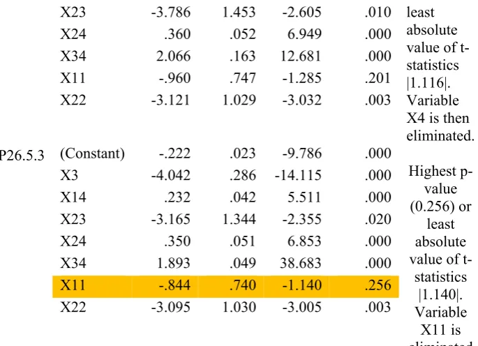
The procedures of eliminating insignificant variables are then carried out as indicated in Table 10 below. Insignificant variables having the highest p-value or the least absolute value of the t-statistics will be eliminated. It can be seen that variables (X13, X4, and X11) are subsequently to be

removed since having p-values of more than 0.05, and hence they are not significant. Table 11 depicts the final matrix for the best model whereby all the remaining variables in the model are significant with their p-values less than 0.05 (α≤ 5%).

Table 10: Insignificant Variables Eliminated From Model P26.5.0

Models

Unstandardized Coefficients

t Sig. Action

Taken B

Std. Error

P26.5.1

(Constant) -.113 .101 -1.120 .265

Highest p-value (0.795) or least absolute value of

t-statistics |0.261|. Variable X13 is eliminated

X3 -4.953 .891 -5.561 .000

X4 -.021 .018 -1.122 .264

X13 -.993 3.807 -.261 .795

X14 .254 .072 3.533 .001

X23 -2.707 4.385 -.617 .538

X24 .343 .083 4.158 .000

X34 2.067 .164 12.634 .000

X11 -.949 .751 -1.264 .209

X22 -3.126 1.033 -3.024 .003

P26.5.2

(Constant) -.112 .101 -1.115 .267

Highest p-value (0.267) or

X3 -4.975 .883 -5.631 .000

X4 -.020 .018 -1.116 .267

X23 -3.786 1.453 -2.605 .010 least absolute value of t-statistics |1.116|. Variable X4 is then eliminated.

X24 .360 .052 6.949 .000

X34 2.066 .163 12.681 .000

X11 -.960 .747 -1.285 .201

X22 -3.121 1.029 -3.032 .003

P26.5.3 (Constant) -.222 .023 -9.786 .000

Highest p-value (0.256) or

least absolute value of

t-statistics |1.140|. Variable

X11 is eliminated

X3 -4.042 .286 -14.115 .000

X14 .232 .042 5.511 .000

X23 -3.165 1.344 -2.355 .020

X24 .350 .051 6.853 .000

X34 1.893 .049 38.683 .000

X11 -.844 .740 -1.140 .256

X22 -3.095 1.030 -3.005 .003

It can also be seen from Table 11 that only one single variable (X3), four first order interaction variables (X14, X23, X24, X34), and one variable of the polynomial (quadratic) term (X22).

Table 11: Correlation Coefficient Matrix of Best Model P26.5.3

Model P26.5.3

Unstandardized Coefficients

t Sig. B

Std. Error

(Constant) -0.222 0.023 -9.776

4.752x10 -17

X3 -4.090 0.284 -14.418 3.352x10 -28

X14 0.186 0.011 16.601 3.389x10 -33

X23 -3.452 1.321 -2.613 1x10-2 X24 0.400 0.026 15.297 3.067x10

-30

X34 1.909 0.047 40.677 3.436x10 -73

X22 -4.136 0.477 -8.667 2.135x10

-14

3.3 Best Model Regression Equation

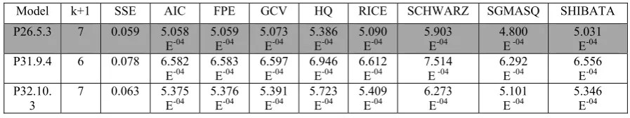
Table12. Comparisons of the Best PR Models Using Newton’s Equation

Model k+1 SSE AIC FPE GCV HQ RICE SCHWARZ SGMASQ SHIBATA P26.5.3 7 0.059 5.058

E-04 5.059 _E-04 5.073 _E-04 5.386 _E-04 5.090 _E-04 5.903 _E-04 4.800 _E -04 5.031 _E-04 P31.9.4 6 0.078 6.582

E-04 6.583 _E-04 6.597 _E-04 6.946 _E-04 6.612 _E-04 7.514 _E -04 6.292 _E -04 6.556 _E-04 P32.10.

3

7 0.063 5.375

E-04 5.376 _E-04 5.391 _E-04 5.723 _E-04 5.409 _E-04 6.273 _E-04 5.101 _E -04 5.346 _E-04

The goodness-of-fit tests comprises of the randomness test and normality test. Randomness test is to determine that the residuals are normally distributed and normality test on the Kolmogorov-Smirnov statistics is to ensure that the normality assumptions are not violated. Since the sample size is 130, the random statistic, R is based on the normal (z) distribution. The null hypothesis is accepted since model P26.5.3 has zero mean of the residuals as shown by the scatterplot of the standardized residuals in Table 13. This implies that the residuals are independent and randomly distributed.

Table 13: Scatterplot and Histogram of the Regression Standardized Residuals.

With a significance level of more than 0.05 (α>0.05), the normality test on the residuals gave the Kolmogorov-Smirnov statistics (0.192) of p-value (0.052) >0.05. From the good-of-fit tests and the plots, the assumptions of randomness and normality of the residuals have therefore been satisfied.

The best polynomial regression model is thus given by Table 11 as:-

34 1.909X 24

0.400X 23

3.452X 14

0.186X 2

4.136X -3 4.09X --0.22 26.5.3

P  2     (7)

Substituting the defined variables back into equation (7), the best model equation is thus:

b 1.909D T

m 0.400D /T

b D m 3.452D -T t 0.186D )

m 4.136(D

-/T b 4.09D --0.22 26.5.3

P  4.5 2 3.7 4.5  4.5  (8)

4. DISCUSSIONS AND CONCLUSIONS

Power Transformation in the form of integers is executed to normalize and linearize the data sets. The resultant model equation has polynomial characterization greater than 2. Previous studies had indicated that complexities of using polynomial regression in regression algorithm where higher orders of the polynomials are concerned (Dam et al., 2000; Ekpenyong et al., 2008). The polynomial relationships of the independent variables with the dependent can be transformed using the p-value method of the normality tests on the variables. Remedial techniques in minimizing multicollinearity effects are applied to obtain a robust model, further followed by the elimination of insignificant variables in the model. The eight selection criteria is effective in identifying the best model, where formally the criteria used is based on the R2 _{or the adjusted-R}2

for model selection. Comparisons between the Newton’s multiple regression models by Noraini et al.(2008) and Noraini et al.(2010(b)), based on the least 8SC, have appeared to represent an improved estimation using polynomial regression models (PRM) for volumetric stem biomass. Diameters at the base, middle, top and tree height have again signified as the main contributors towards the stem volume estimation.

Acknowledgements

The authors would like to acknowledge the financial support from Universiti Malaysia Sabah in this study.

REFERENCES

Akaike, H. (1970). “Statistical Predictor Identification”. Annal Institute of Statistical Mathematics 22, pp.203-217. Akaike, H. (1974). “A New Look at model Statistical Identification”. IEEE Trans Auto Control 19, pp.716-723. Bechtold, W.A. (2004). “Largest-crown width prediction models for 53 species in the western United States”. West

Journal Appl. Forest 19(4), pp.245-251.

Ashish, K.S. & Muni, S. (1990). Regression Analysis:Thyeoriy, Methods and Applications. Springer, New York. Coakes, S.J. & Steed, L. (2007). SPSS:Analysis without anguish:version 14.0 for windows. Wiley, Sydney.

Dam, J.S., Dalgaard, T., Fabrcius, P.E. & Andersson-Engels, S. (2000). Multiple Polynomial Regression Method for Determination of Biomedical Optical Properties from Integratin Sphere Measurements. Applied Optics 39(7). Devore, J. & Peck, R. (1993).Statistics, the Exploration and Analysis of Data. Wadsworth, California.

Ekpenyong, J.E., Okonnah, M.I. & John E,D. (2008). Polynomial (Non-Linear) Regression Method for Improved Estimation Based on Sampling. Journal of Applied Sciences 8(8):1597-1599.

Fuwape, J.A., Onyekwelu, J.C. & Adekunle,V. A.J. (2001). “Biomass Equations and Estimation for Gmelina Arborea and Nauclea Diderrichii Stands in Akure Forest Reserve”. Biomass and Bioenergy21, pp.401-405.

Golub, G.H., Heath, M. & Wahba, G. (1979). Generalized cross-validation as a method for choosing a good ridge parameter. Technometrics 21, pp.215-223.

Gujarati, D.N. (2006). Essential of Econometrics. 3rd _{Edition. New York. McGraw Hill Companies, Inc.}

Hannan, E.J. & Quinn, B.G. (1979). “The Determination of the Order of an Autoregression”. Journal of Royal Statistics Society, Series 41(B), pp.190-195.

Hasenauer, H. (eds.). (2006). “Concepts within Tree Growth Modelling”. Sustainable Forest Management. Springer. New York.

Noraini, A., Zainodin, H.J. & Nigel Jonney J.B. (2008). “Multiple Regression Models of the Volumetric Stem Biomass”. WSEAS Transactions on Mathematics7(7) pp.492-502.

Ramanathan, R. (2002). Introductory Econometrics with Applications. 5th Ed. South-Western, Thomson Learning, Ohio.

Rice, J. (1984). “Bandwidth Choice for Nonparametric Kernel Regression”. Annals of Statistics 12, pp.1215-1230. Noraini, A., Amran Ahmed & Zainodin, H.J. (2010)(a). ”Urban Forest Sustainability using MR Models”. American

Journal of Environmental Sciences(submitted for publication).

Noraini, A., Zainodin, H.J. & Amran Ahmed. (2010)(b). “Comparisons between Huber and Newton’s Multiple Regression Models for Stem Biomass Estimation”. Malaysian Journal of Mathematical Sciences(submitted for publication).

APPENDIX

All Possible Polynomial Models

P1 1 2 1 11 1 1 0

1     X   X 

V P2 2 2 2 22 2 2 0

2     X   X 

V P3 3 2 3 33 3 3 0

3     X   X  

V P4 4 2 4 44 4 4 0

4     X   X 

V P5 5 2 2 22 2 1 11 2 2 1 1 0

5     X   X   X   X  

V P6 6 2 3 33 2 1 11 3 3 1 1 0

6     X   X   X   X 

V P7 7 2 4 44 2 1 11 4 4 1 1 0

7     X   X   X   X 

V P8 8 2 3 33 2 2 22 3 3 2 2 0

8 X X X X

V        

P9 9 2 4 44 2 2 22 4 4 2 2 0

9     X   X   X   X 

V P10 10 2 4 44 2 3 33 4 4 3 3 0

10     X   X   X   X 

V P11 11 2 3 33 2 2 22 2 1 11 3 3 2 2 1 1 0

11     X   X   X   X   X   X 

V P12 12 2 4 44 2 2 22 2 1 11 4 4 2 2 1 1 0

12     X   X   X   X   X   X 

V P13 13 2 4 44 2 3 33 2 1 11 4 4 3 3 1 1 0

13     X   X   X   X   X   X 

V P14 14 2 4 44 2 3 33 2 2 22 4 4 3 3 2 2 0

14     X   X   X   X   X   X 

V P15 15 2 4 44 2 3 33 2 2 22 2 1 11 4 4 3 3 2 2 1 1 0 15 X X X X X X X X V                     P16 16 12 12 2 2 22 2 1 11 2 2 1 1 0

16     X   X   X   X   X 

V P17 17 13 13 2 3 33 2 1 11 3 3 1 1 0

17   X  X  X  X  X 

V P18 18 14 14 2 4 44 2 1 11 4 4 1 1 0

18   X  X  X  X  X 

V P19 19 23 23 2 3 33 2 2 22 3 3 2 2 0

19   X  X  X  X  X 

V P20 20 24 24 2 4 44 2 2 22 4 4 2 2 0

20   X  X  X  X  X 

V P21 34 34 34 2 4 44 2 3 33 4 4 3 3 0

21   X  X  X  X  X 