MATHEMATICAL MODEL FOR LINEAR ANALYSIS OF THE STABILITY OF A SYSTEM DURING UNIDIRECTIONAL SOLIDIFICATION WITH BUOYANCY AND SMALL SEGREGATION COEFFICIENT

MATHEMATICAL MODEL FOR LINEAR ANALYSIS

OF THE STABILITY OF A SYSTEM DURING

UNIDIRECTIONAL SOLIDIFICATION WITH

BUOYANCY AND SMALL SEGREGATION

COEFFICIENT

Dr. Roopa K.M

Professor, Dept. of Mathematics, Bangalore Institute of Technology, Bangalore, (India)

ABSTRACT

In this study, the stability of a coupled morphological-convective system during unidirectional solidification

with buoyancy is discussed for small segregation coefficient as well as a small wave number. The effects of the

constraints like rotation, permeability and quadratic density profile are investigated by considering linear

theory. Expressions for the growth rate, critical conditions and solutions corresponding to different order of

approximations are determined by using power-series expansion technique with boundary conditions.

Keywords:

Linear Analysis, Buoyancy, Small Segregation Coefficient, Small Wave Number.

I. INTRODUCTION

Three models like rotation, permeability and quadratic density profile are investigated using linear theory in detail. Expressions for the growth rate, critical conditions and solutions corresponding to different order of approximations are determined. The physical configuration (Figure 2.1) consists of a binary-alloy melt which is directionally solidified at constant speed V.

Under the assumptions and approximations [1], [6] and [7], the heat generated at the solidifying front can be neglected and accordingly, it can be presumed that the interfacial perturbations do not give rise to disturbances of the temperature field. Therefore, the temperature field can be considered to be fixed as:

z

G

T

T



₀



(9.1.1)

II. MATHEMATICAL FORMULATION

In this study, the mathematical formulation has been constituted in a frame of reference moving at the velocity V (the crystal growth rate)as given in the following equations [1], [3] and [7]:

The conservation of momentum:

 

    

       

k u

u u u u

g p

z t

0 2

0 V











(9.1.2)

The conservation of solute in the melt:

 

D c

z c V c u t

c _{ }2

       

(9.1.3)

The conservation of mass:

. u = 0 (9.1.4)

Where,

u

is the fluid velocity, p is the reduced fluid pressure, c is the mass concentration of the solute in the

fluid,



0_{is the reference density and}



_{is the kinematic viscosity of the fluid. The diffusion of the solute in the}

solid phase is also neglected. The quadratic density profile is given by:





2

0

f

C c









(9.1.5)

Where,



is the change in the density;



 



0

is the solutal coefficient of expansion;

C

f_{is the concentration of}

the solute in the fluid at the interface.

2.1 Boundary Conditions

Under the assumption, if the density changes upon solidification is negligible, the no-slip condition and the mass

balance condition are:

u



0

(9.1.6) The mean position of the interface is taken as z = h (x, y, t) and the conservation of solute at the interface:

c(1k )( V + h t ) = D(cz  cxhx  cyhy ), where, the subscript denotes the derivative. (9.1.7) The condition of thermodynamic equilibrium:

T = mc + TM [ 1 + L 

K ] , 

   _

 

 K

L γ 1 T mc Gh

T_{0 M}

from (9.1.1) (9.1.8)

Where, m is the liquidus (figure 2.2) slope, TM is the melting point of the pure substance,



is the surface free energy, L is the latent heat and K is twice the mean curvature:















2



32

y 2 x 2

x yy xy y x 2 y

xx

1

h

2h

h

h

h

1

h

1

h

h

h

K



















(9.1.9) Far away from the interface, the velocity field is considered to be bounded and the solute concentration is equal

to

C

s_{, which is the concentration of the solute in the solid phase.}

2.2 Basic State Solution

(i) A planar interface

h



0

(9.1.10), (ii) Zero melt velocity



u



0



(9.1.11)

(iii) The reference temperature of the planar interface:

(9.1.12) ... .. T k mC T M s 

(iv) The solute gradient at the interface:





D V C G s c k k1



(9.1.13)

(v) The concentration field: 

                D

cD _e

G Cs c z V V 1 k (9.1.14)

Where, V

D





is the concentration boundary-layer thickness (9.1.15)

The governing equations (9.1.2) to (9.1.4) are made dimensionless by using the following scales [2] and [4]:

Length:

x





x



,

y





y



,

z





z



,

h





h



; Velocity:

u



V

u



,

v



V

v



,

w



V

w



Pressure: p 2    D V p

; Time: V t D t 

2

; Concentration:

c D G C

c s c _{ }

       V

k _(9.1.16)

The resulting dimensionless equations are:

















          











k

u

u

u

u

u

₂

_*

₂

1

_p

_RC

_c

S

z

-t

(9.1.17)

 

c

2

c

t

c

_

_









  

z

-c

u

(9.1.18); . u= 0 (9.1.19)

D S



: Schmidt number; G

mG

M c

: the Morphological parameter;

R = 4















V

D

D

G

g

c





₌ 3

V

D

D

β

g

)C

1

















k

k

s

(

: the solute Rayleigh number; (9.1.20)

 = 2 M D V LmG T c       

: surface free energy parameter;

s

C

C



_



_



k

k

-

1

*

: Segregation ratio;

The interface

z



h



x,

y,

t



in the dimensionless form are given by: u=0 (9.1.21)







c

k



1



1



1



h

t





c

z



h

x

c

x



h

y

c

y _(9.1.22)











1

2

2

1

2







1

2 2





32

0

1





















  y x x yy xy y x y

xx

h

h

h

h

h

h

h

h

h

h

M

c

--- (9.1.23)

From (9.1.19) and (9.1.21), we have D w = 0 at the interface (9.1.23a)

Far away from the interface (i.e. as

z





) the conditions are:





u

, c = 1 …… (9.1.24)

Thus, the dimensionless basic state solution:





u

x

p

z

u

u

u

S

1 2

t











































_u

(9.1.28)





v

y

p

z

v

t

v

S





2





































1

_u

_v

(9.1.29)





2 * 2

1 c RC w z p z w w t w

S  

                

_u

(9.1.30) The pressure, in (9.1.28) - (9.1.30), is eliminated by applying the operator curl twice on (9.1.17). The resulting equation in the vertical component of velocity is given by:





2

4

_RC

*

_c

2

2

w

2

t

S

2 1













































w

w

z

w

1

_u

(9.1.31) Where, 2 2 2 2 2 1 y x       

is the two - dimensional Laplacian operator

III. LINEAR STABILITY ANALYSIS

The stability of the melt for infinitesimal perturbations is discussed. Widely used and accepted method is employed in the study [7]. The Leading-order solutions as well as corrections to the leading-order solutions are computed by considering higher order approximations. To introduce disturbances to the basic state as follows:



u,

v,

w

 



0,0,0

 



ε

U,

V,

W



_(9.1.32)

H

ε

0

h





_(9.1.33)

C ε e 1

c  z

(9.1.34) Substituting the above equations such as (9.1.32), (9.1.33), (9.1.34) with (9.1.14), (9.1.31), (9.1.21) to (9.1.25)

and then linearising with respect to



, we get the set of differential equations in terms of



. The normal modes

for each of the dependent variable as



    

t σ

e

y

x,

g

z

F

t

z,

y,

x,

f



_(9.1.35)

Where,

g

 

x,

y

satisfies:

g

g

a

g

2

yy

xx







_(9.1.36)

And the growth rate



determines the stability of the marginal state. In (9.1.36), ‘a’ is the horizontal wave number. By equating the coefficient of from the resulting equation, to obtain the system of equations as follows:



_{2C 2Ce}z



a RC W a z d d W a z d d z d d W a z d d σ

S * 2

2 2 2 2 2 2 2 2 2 2 1   _{ }                                      Or



1

e



C

a

2RC

W

σ

S

a

z

d

d

S

z

d

d

a

z

d

d

1 2 1 * 2 _z

2 2 2 2 2   

_

_

_













_

_

_









_

(9.1.37) z

We

C

σ

a

z

d

d

S

z

d

d

1 2

2 2  

_













_

_

_

(9.1.38) The associated boundary conditions at the undisturbed interfacial position:

z = 0,

0 z d dW

W 

  

1 k C σ k



H 0 z

d

dC_{    }

(9.1.40)



1



1









2



0

H

a

C

H

M

_(9.1.39)

Far away from the interface as z,

|

W

|





,

C



0

(9.1.41) By solving (9.1.40), obtained the linearized thermodynamic equilibrium equation for the interfacial

Perturbation i.e. H, where





1 2

1











M

a

C

H

(9.1.42)

From (9.1.42), it is clear that if M0, then H is forced to tend to be zero and this corresponds to the unperturbation state. This result is very much consistent with (9.1.20). In other words, there will be no morphological instability if the under cooling is set equal to be zero. Further, the substitution of (9.1.42) with (9.1.40) yields the equation of the mass conservation of solute at the interface:





_





_

0

1

1

2







1













_

M

a

C

C

z

d

dC

k

k

(9.1.42) Where, due to an interfacial-shape change, the third term represents the perturbation in the concentration field.

From (9.1.42), it follows that near the critical value for the onset of convection for which M1, the third term

will be proportional to 2

1

a

. It is clear that, if the wave number is sufficiently small, then this term would

definitely dominate the diffusion term dz

dC

and this is a singular perturbation. Then from Physics, it follows

that, the dimensional wavelength or the characteristic cell size of an interfacial perturbation is a

2 V

D 

 

(9.1.43)

From (9.1.43), it is implied that decrease in ‘a’ leads to increase in the wavelength. In other words, the cell size

exceeds the diffusional width

V

D

for very small values of ‘a’. Thus, the cell gets elongated at the onset of instability (M=1).

In the further analysis, the whole problem is rescaled for k<<1 under the assumption that ‘a’ is also very smaller

than 1. Thus, to introduce:

k

k

~

2

a



_and  2~

a _(9.1.44)

The governing system of equations under this new scaling becomes:



1

S

σ



W

2RC

a



1

e



C

a

z

d

d

S

z

d

d

a

z

d

d

1 2 1 * 2 z

2 2 2 2 2

 



_

_

_













_

_

_









_

~

(9.1.45)

 

₁

_σ

_C

_We

z

a

z

d

d

z

d

d

2

2 2

















_

_

_

_~

(9.1.46)

Together with the conditions at z=0:

0 z d dW

W 

(9.1.47)





_

 

_

0

Γ

a

1

M

C

k

σ

a

-C

k

a

1

z

d

dC

2 1 2

2













~

_

~

~

(9.1.48)

3.1 The Solution Procedure

To introduce power-series expansion for all the dependent variables of the problem under consideration as follows:













2 ₁

0

a

W

W

W

_;





2 ₁









0

a

C

C

C

_(9.1.50)

By substituting power-series expansion of (9.1.50) with (9.1.45) to (9.1.49) and also equating the like powers

of

a

2 to get a set of differential equations corresponding to different order of approximations, the leading order will be:

0

W

S

z

d

d

z

d

d

0 1 3 3















_









 (9.1.51) z e W C 1 z d d z d d 0 0         _ (9.1.52)

With

W

0



DW

0



0

_{at z=0;}

|

W

0

|





_{as z} _;



D



1



C

0



0

_{at z=0;}

C

0



0

_{as z} _(9.1.53)

The corresponding solutions are:

W

0



0

_(9.1.54)

z

Ae

C

0





_{, where A is an arbitrary constant (9.1.55)}

The equations at

 

2

a

O

_are,



e

e



A

C

2R

W

S

z

d

d

z

d

d

* 2_{z z}

1 1 3 3   

_

_

_

_











_









(9.1.56)

 

_{1 σ C We}z

C 1 z d d z d d 1 0 1           _ ~ (9.1.57) With

0

dz

dW

W

1

1





at z=0;

|

W

1

|





_,

C

1



0

_{as z}_;

 





0

1

Γ

a

M

A

k

σ

A

k

C

dz

dC

2 1 1 1















~

_

~

~

at z=0 (9.1.58) The corresponding solutions are:

z z z

e

A

e

A

e

A

A

W

14 2 13 S 12 11 1   











_(9.1.59)

Where, S RC A 4 7 A11 *

,







S 1



2S 1



7 S 3 7S 2A A 11

12 _{ }

 

’ 7



2S 1



A

A 11

13 _

,



S 1



A 7 8

A 11

14 _

And

 





_

_

_

_

 





24



2S

1



e

A

1

S

e

A

e

1

2S

1

S

2

S

A

ze

σ

1

A

A

Be

C

z z z z

z 15 3

2 15 S 1 S 2 3 15 11 1





































~

     (9.1.60)

Where,

S

*

RC

A

₁₅



(9.1.61)

Now substituting and simplifying the expression for

C

1 _{into the last equation of (9.1.58), we find the expression}

for the growth rate:

















k



















































Although the general form of



corresponding to linear and quadratic density profiles is same and also the influence of quadratic profile is clearly seen in the second part of the first term, in the absence of gravity (i.e.

R=0) in the limit of M=1 and

a

2 being very small then, the equation (9.1.62) reduces to:



1

M



a

a

k

σ

_

_

1 2

_

4

_

_

(9.1.63) This result is identical to that of linear density profile (since R=0) and also, this expression is identical to that of

[5] and [7]. From (9.1.63), we compute the critical values of R and by setting





0

.Thus,

















































_*1 _1_{1 2}2 ₄

a

a

M

1

a

M

1

C

5

S

1

6

R

k

(9.1.64)

and the condition

0

da

dR

2



for optimality yields:





_

_









_

_

















  2

2 1 1

*

M

1

Γ

k

1

5

S

1

6

C

R

_c

(9.1.65)

Where,

2 c

a

_{satisfies the equation:}



2

 

a

2 2



2

M

1



a

2



M

1



1



M

1





0

(9.1.66)

Solving (9.1.66), we obtain

a

M



M

1



2 1 1 1 2

c







 

(9.1.67)

Equation (9.5.65), in the limit M0, reduces to





* 1 c

C

5

S

1

6

R







(9.1.68)

From (9.1.68), it is evident that

R

c_{depends on segregation ratio parameter and the Sekerka number. When the}

density profile is quadratic, there is a drastic change in the value of

R

c_{. Also in the}Ltk0_, C* _becomes

infinite so that

R

c



0

_.

From the definitions of

M

1and



, both are inversely proportional to the solute concentration

C

S_{. Therefore,}

increase in

C

S_{, the value of wave number also increases as well as the cell structure will get contracted in case}

of a pure substance. Obviously,

C

S



0

_{and a=0 and that corresponds to a planar interface.}

Suppose, we make an approximation that R=0, near M=1, then clearly M -1= O (a2) and from (9.1.63):













k



2 4

a

a

1

M

~

_{(Since M~1) (9.1.69)}

To apply this approximation to (9.1.69), we obtain:



12



2 c

M

1

M

1

M

a









_

    

  2

1 M ~

(9.1.70) As the asymptotic expansions considered in this study is valid only for a2<<1 and hence from (9.1.70), we get:

1 2

1 M _

    

 

&





1 1 M 4

1  2

 

k

(9.1.71)

IV. RESULTS AND DISCUSSIONS

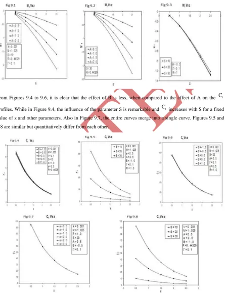
In Figures 9.1 to 9.3, the profiles of

W

1_{are presented for different combinations of the parameters. While,}

Figure 9.1 predicts the variation of

W

1 _{w.r.t. A for k=0.001, M=1.025, S=10, R=0.44329 and}





0

.

1

_{. It is}

observed that,

W

1 _{decreases with z and is negative for all the combinations.}

From Figures 9.4 to 9.6, it is clear that the effect of B is less, when compared to the effect of A on the

C

1

profiles. While in Figure 9.4, the influence of the parameter S is remarkable and

C

1 _{increases with S for a fixed}

value of z and other parameters. Also in Figure 9.7, the entire curves merge into a single curve. Figures 9.5 and 9.8 are similar but quantitatively differ from each other.

While in Figure 9.9, the effect of



is almost nil on the profile C1. In Figure 9.10, the graph of Rc vs S is

In Figure 9.11, the graph of

2 c

a

_vs

_

_{is linear whereas in Figure 9.12, the curves depict the effect of}

_

_on

a

2_c

for a fixed value of M. Further, the effect of M is to increase the value of

2 c

a

for fixed values of the parameters under consideration.

In Figure 9.13, the variation of R with respect to M is presented. While Figure 9.14 predicts that R decreases with S for M=0.

Note: In all the graphs, R = RC* and Rc = Rc C*.

V. CONCLUSION

and for small wave number. Since, linear stability analysis has its own limitations; the nonlinear analysis would be recommended.

ACKNOWLEDGEMENT

The support from Dr.A.M. Ramesh, Senior Scientific Officer, Srinivasu V.K, Scientific Officer and Umesh Ghatage, Scintific Officer from Karnataka Science and Technology Academy is gratefully acknowledged.

REFERENCES

[1] JOSEPH, D.D., 1976. Stability of fluid motions I & II. Springer Tracts Natural Phil. 27, ch. X, XI.

[2] MAURICE HOLT, 1961. Dimensional Analysis, Sec. 15 in Victor L. Streeter (ed.), Handbook of Fluid Dynamics, McGraw-Hill Book Company, New York.

[3] RIAHI, D.N., 1993. Effect of rotation on the stability of the melt during the solidification of a binary alloy. Acta Mechanica 99, 95.

[4] SEDOV, L.I., 1959. Similarity and dimensional methods in Mechanics (Trans. By M. Friedman), Acad. Press Inc., New York.

[5] SIVASHINSKY, G.I., 1983. On cellular instability in the solidification of a dilute binary alloy. Physica 8D, 243.

[6] SRIMANI, P.K., 1981. Finite amplitude cellular convection in a rotating and non-rotating fluid saturated porous layer. Ph.D. Thesis, Bangalore University, India.