Toward Realistic Modeling Of Catalytic Surfaces: From First Principles To Machine Learning

(1)

University of Pennsylvania University of Pennsylvania

ScholarlyCommons

Publicly Accessible Penn Dissertations

2019

Toward Realistic Modeling Of Catalytic Surfaces: From First

Principles To Machine Learning

Robert Bruce Wexler

University of Pennsylvania, [email protected]

Follow this and additional works at: https://repository.upenn.edu/edissertations Part of the Physical Chemistry Commons

Recommended Citation Recommended Citation

Wexler, Robert Bruce, "Toward Realistic Modeling Of Catalytic Surfaces: From First Principles To Machine Learning" (2019). Publicly Accessible Penn Dissertations. 3517.

(2)

Toward Realistic Modeling Of Catalytic Surfaces: From First Principles To

Machine Learning

Abstract Abstract

Computational catalyst design has the potential to revolutionize the energy and chemical industries by alleviating their reliance on fossil fuels, precious metals, and toxic elements. Despite recent advances in understanding catalytic trends, e.g. the chemisorption scaling relations and the d-band model, the description of catalytic surfaces has, for the most part, been far from realistic. It is well known that surfaces can undergo reconstruction where the structure and composition of the surface differs from that of the bulk and the nature of this reconstruction depends on the temperature, pressure, and chemical potentials of the elements in the system. Since catalytic transformations, i.e. bond breaking and

formation, occur at the surface, an accurate picture of surface structure and composition is vital. In this thesis, we apply and develop state-of-the-art computational methods for studying the reconstruction of catalytic surfaces and investigate the effect of surface reconstruction on catalysis. First, we show using ab initio thermodynamics that the surfaces of nickel phosphide catalysts for the hydrogen evolution reaction (HER) are P-enriched, which was not previously considered in computational studies. Building on this discovery, we reevaluate the HER mechanism on Ni2P and Ni5P4 and find that P sites are the key to their catalytic activities. While the P sites on Ni2P are highly active toward the HER, they are not stable at conditions suitable for commercial electrolyzers. Under these conditions, the stable surface of Ni2P binds hydrogen too strongly at Ni sites. We demonstrate that these Ni sites can be activated by doping the surface of Ni2P with S, Se, and Te. Additionally, using tree-based machine learning methods, we reveal that nonmetal dopants induce a chemical pressure-like effect on the Ni sites, changing their reactivity through compression and expansion. Finally, we develop a software package for ab initio grand canonical Monte Carlo that automatically predicts surface phase diagrams. The results presented herein provide strong motivation and a methodological foundation for moving toward more realistic modeling of heterogeneous catalysts. Degree Type Degree Type Dissertation Degree Name Degree Name

Doctor of Philosophy (PhD)

Graduate Group Graduate Group Chemistry

First Advisor First Advisor Andrew M. Rappe

Second Advisor Second Advisor Jeffrey G. Saven

Keywords Keywords

Computational catalysis, Density functional theory, Grand canonical Monte Carlo, Machine learning, Nickel phosphides, Surface chemistry

(3)

TOWARD REALISTIC MODELING OF CATALYTIC SURFACES: FROM FIRST PRINCIPLES TO MACHINE LEARNING

Robert B. Wexler A DISSERTATION

in Chemistry

Presented to the Faculties of the University of Pennsylvania in

Partial Fulfillment of the Requirements for the Degree of Doctor of Philosophy

2019

Supervisor of Dissertation

Dr. Andrew M. Rappe

Blanchard Professor of Chemistry, and

Professor of Materials Science and Engineering

Graduate Group Chairperson

Dr. David W. Christianson

Roy and Diana Vagelos Professor in Chemistry and Chemical Biology

Dissertation Committee

Dr. Jeffrey G. Saven, Professor of Chemistry

Dr. Christopher B. Murray, Richard Perry University Professor of Chemistry and Materials Science and Engineering

(4)

c

COPYRIGHT

2019

(5)

(6)

ACKNOWLEDGEMENTS

I would like to thank Prof. Andrew M. Rappe for motivating me to set lofty goals, be-ing understandbe-ing in difficult times, encouragbe-ing me to think creatively, and providbe-ing me with opportunities to develop a well-rounded set of research skills.

I would also like to thank Dr. J. Mark P. Martirez for teaching me about ab initio

thermodynamics and electrocatalysis, answering my (many) questions, mentoring me in my first graduate research project, and advocating for me.

I would like to express my appreciation to Prof. G. Charles Dismukes for sharing his unique perspective on electrocatalyst design, supporting me in my job applications, and imparting helpful career and life advice. Also, to Dr. Anders B. Laursen for stimulating conversations and our fruitful collaboration.

I would like to offer my thanks to the members of the Rappe group, past and present, for countless insightful discussions, their willingness to assist me, and the lasting friendships. To Mr. Tian Qiu for helping me developab initio grand canonical Monte Carlo and giving of your time so generously. To Dr. Arvin Kakekhani for deepening my understanding of catalysis.

(7)

ABSTRACT

Robert B. Wexler

Dr. Andrew M. Rappe

Computational catalyst design has the potential to revolutionize the energy and chemical industries by alleviating their reliance on fossil fuels, precious metals, and toxic elements. Despite recent advances in understanding catalytic trends, e.g. the chemisorption scaling relations and the d-band model, the description of catalytic surfaces has, for the most part, been far from realistic. It is well known that sur-faces can undergo reconstruction where the structure and composition of the surface differs from that of the bulk and the nature of this reconstruction depends on the temperature, pressure, and chemical potentials of the elements in the system. Since catalytic transformations, i.e. bond breaking and formation, occur at the surface, an accurate picture of surface structure and composition is vital. In this thesis, we apply and develop state-of-the-art computational methods for studying the reconstruction of catalytic surfaces and investigate the effect of surface reconstruction on catalysis. First, we show using ab initio thermodynamics that the surfaces of nickel phosphide catalysts for the hydrogen evolution reaction (HER) are P-enriched, which was not previously considered in computational studies. Building on this discovery, we reeval-uate the HER mechanism on Ni2P and Ni5P4 and find that P sites are the key to

their catalytic activities. While the P sites on Ni2P are highly active toward the

(8)

these conditions, the stable surface of Ni2P binds hydrogen too strongly at Ni sites.

We demonstrate that these Ni sites can be activated by doping the surface of Ni2P

(9)

LIST OF TABLES

TABLE 2.1 : ZPE, standard entropy, and integrated heat capacity of H2

and H2O at 298 K and 1 bar in units of eV. . . 42

TABLE 3.1 : Calculated L¨owdin charges for the surface P atoms for some of the stable reconstructions of Ni2P and Ni5P4. . . 82

TABLE 4.1 : Free energy of H adsorption on selected surface sites of Ni2P(0001)

and Ni5P4(000¯1) in equilibrium with 1 M Ni2+ or Ni(s), and

1 M PH3 or 1 M H3PO4 at 298.15 K,U = 0 V, and pH = 0. 95

TABLE A.1 : Calculated and experimental bulk parameters in ˚A . . . 146 TABLE A.2 : Calculated L¨owdin charges for the surface atoms for the stable

surface reconstructions and some of the bulk-derived termina-tions of Ni2P and Ni5P4(0001) and (000¯1). . . 153

TABLE B.1 : Experimental standard formation free energy of solid and aque-ous Ni and P species. (1) n corresponds to the stoichiometric coefficients in Eq. B.4. . . 158 TABLE B.2 : Free energy of Ni2P(0001) surfaces in equilibrium with 1 M

Ni2+ _{or Ni(}_s_{), and 1 M PH}

3 or 1 M H3PO4 at 298.15 K.n

cor-responds to the number of atoms removed from the reference surface, Ni2P-Ni3P2+P, to obtain a given surface. All energies

(15)

TABLE B.3 : Free energy of Ni5P4(0001) surfaces relative to Ni5P4-Ni4P3(0001)

in equilibrium with 1 M Ni2+ _{or Ni(}_s_{), and 1 M PH}

3 or 1 M

H3PO4 at 298.15 K. All energies are reported in eV. . . 166

TABLE B.4 : Free energy of Ni5P4(000¯1) surfaces relative to Ni5P4-Ni4P3(000¯1)

in equilibrium with 1 M Ni2+ _{or Ni(}_s_{), and 1 M PH}

3 or 1 M

H3PO4 at 298.15 K. All energies are reported in eV. . . 169

TABLE C.1 : Standard oxidation/reduction free energy of nonmetal stan-dard states to form most stable phases at U = 0 V vs. SHE and pH = 0 (∆G◦_A(std)_/_H

xAOzy) (1). All energies are reported in

eV/molecule. . . 183 TABLE C.2 : DFT-calculated free energy of substituting P with other

non-metals relative to their standard states (∆Gdsrp,A−∆Gdsrp,X).

All energies are reported in eV/atom. Note that DFT-PBE is known to overbind O2 by 0.80 eV (2) and N2 by 0.50 eV (3).

We corrected this by performing DFT total energy calcula-tions for triplet O and quadruplet N and then adding their experimental binding energies (5.16 eV/O2 and 9.81 eV/N2).

For example, for O2 we usedEO2 = 2E

DFT

O +E

exp

bind. For O2 and

N₂, we also included the experimental integrated heat capacity and the standard entropy of the gas. . . 184

TABLE D.1 : Convergedk-point grids and energy cutoffs for bulk Ag, Ag₂O, and O₂ . . . 189 TABLE D.2 : Lattice constants for bulk Ag and Ag₂O in ˚A. . . 190 TABLE D.3 : Optimal parameters of the random forest regressor implemented

(16)

LIST OF ILLUSTRATIONS

FIGURE 1.1 : Classic examples of surface reconstruction, (a) Si(111)-7×7 and (b) Au(110)-1×2. Blue and yellow spheres correspond to silicon and gold atoms, respectively. Si(111)-7×7 has an-gle cavities (red), rest atoms (green), dimers (magenta), and adatoms (black). The side view is obtained by cutting the top view along the dashed line and then rotating about it by 90◦. Half of the surface unit cell of Si(111)-7×7 has a stacking fault arrangement whereas the other half does not. Au(110)-1×2 has missing rows along [100] that repeat every two surface unit cells. . . 7

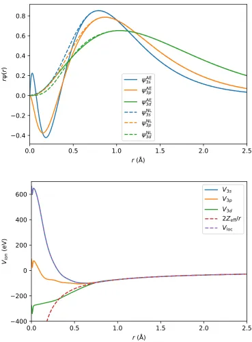
FIGURE 2.1 : Pseudopotential of P. (Top) All-electron (AE) wave func-tions and nonlocal (NL) pseudo-wave funcfunc-tions of the P 3s, 3p, and 3d states. NL pseudo-wave functions are nodeless and smoother than the AE wave functions. (Bottom) Ionic pseudopotentialsV3l, true atomic potential (shaded red), and

local potential Vloc. Ionic pseudopotentials do not diverge as

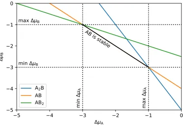
r →0 and are smoother than the true atomic potential. . . 21 FIGURE 2.2 : Bulk phase diagram of a hypothetical binary compound AxBy

with three stable compositions A2B, AB, and AB2. Dotted

(17)

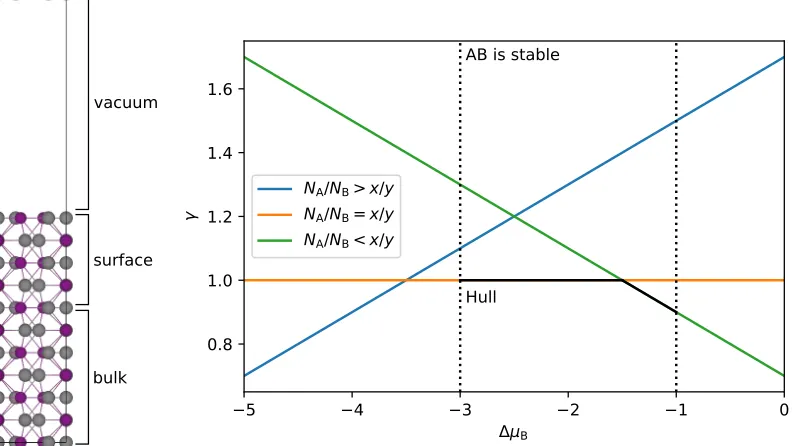
FIGURE 2.3 : Slab model (left) and surface phase diagram (right) of a hy-pothetical binary compound AxBy. (Left) Silver and purple

spheres correspond to A and B, respectively. (Right) Surface energyvs.the relative chemical potential of B. Three surface compositions are shown, two of which (orange and green) are stable in the region of ∆µB where bulk AB is stable. . . 34

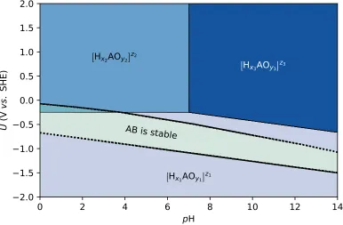
FIGURE 2.4 : Pourbaix diagram of a hypothetical element A with three stable aqueous phases. Dotted lines enclose the region of U

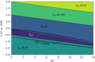
and pH where AB is stable. . . 37 FIGURE 2.5 : Aqueous surface phase diagram of a hypothetical binary

com-pound AxBy. Five surface phases are shown, three of which

(dark green, purple, and blue) are stable in the region of U

and pH where AB is stable. The composition of the surface layer is defined relative to that of some reference (ref) Sref,

e.g. Sref-B+H corresponds to a surface that has one B

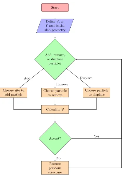
re-moved and one H adsorbed. Dotted lines correspond to the region of U and pH where AB is stable. . . 41 FIGURE 2.6 : Schematic of the grand canonical ensemble. The system

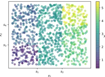
(with energy E, number of particles N, and volume V) is in contact with a reservoir (with energy E0 and number of particles N0) with which it can exchange heat ∆E and par-ticles ∆N. . . 48 FIGURE 2.7 : Flow chart of a GCMC simulation. . . 52 FIGURE 2.8 : Data used to grow the DT in Fig. 2.9. The data consists of

two inputsx1 and x2, one responsey, and 1000 observations.

(18)

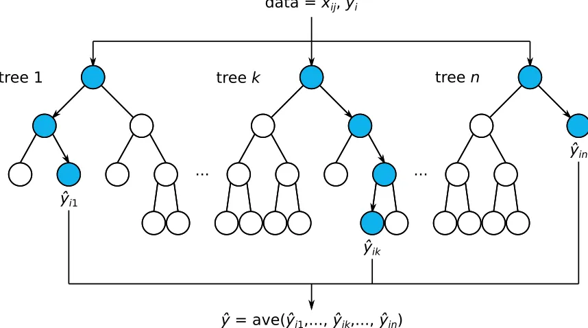
FIGURE 2.9 : DT for the data shown in Fig. 2.8. Questions (inequalities) split the data into groups, which are further split into sub-groups by follow-up questions. Predictions are made by pass-ing new observations from question to question until they are assigned a ¯y. . . 58 FIGURE 2.10 :Schematic of a RF, which consists ofn DTs trained on

differ-ent subsets of the observations i and inputsj. Circles corre-spond to questions. The predicted response ˆyof a new obser-vation is calculated by passing it through each DT, shown as blue circles connected by arrows, and averaging their responses. 61

FIGURE 3.1 : Crystal structure of (a) Ni2P and (b) Ni5P4, highlighting

(19)

FIGURE 3.2 : Surface crystal structure of Ni2P(0001) with either a (a) Ni3P

or (b) Ni3P2 termination. Only the atoms of the outermost

layers are clearly shown. Structural insets highlight the basic subunits of each surface. Red lines outline the√3×√3R30◦ supercells. (c) Surface phase diagram for Ni2P(0001) as a

function of ∆µP(eV). Surface energies are reported in J/m2.

Dashed gray vertical lines border the bulk stability region for Ni2P. . . 71

FIGURE 3.3 : Surface crystal structure for bulk-derived terminations and reconstructions of Ni5P4(0001) and (000¯1). (a) Bulk

layer-ing in Ni5P4. (b) Bulk-like (0001) terminations Ni3P2 (top),

Ni3P3 (middle), and Ni4P3(bottom) with shaded regions

cor-responding to the insets highlighting important structural features. (c) Stable (0001) reconstructions Ni5P4-Ni3P3+2VP+P

(left) and Ni5P4-Ni4P3+3P (right). (d) Bulk-like (left) and

reconstructed (right) Ni5P4-Ni4P3+3P(000¯1). . . 77

FIGURE 3.4 : Surface phase diagram for Ni5P4(0001) and (000¯1) surfaces

as a function of ∆µP(eV). ΩT+Bcorresponds to the combined

surface energies (J/m2_{) of the top (T) and bottom (B)}

sur-faces of (a) Ni3P2(0001), (b) Ni3P3(0001), (c) Ni4P3(0001),

and (d) Ni4P3(000¯1) and their respective reconstructions.

Shaded areas denote regions of ∆µP where certain

(20)

FIGURE 4.1 : (A) Surface phase diagram of Ni2P(0001) in equilibrium with

1 M Ni2+ _{or Ni(}_s_{), and 1 M PH}

3 or 1 M H3PO4 at 298.15 K.

(B)-(D) show the evolution of the surface through adsorption-desorption equilibrium of P. P dissolves off the surface as phosphates (B). As the potential is lowered it redeposits as phosphines (C), up to a point where PH3 becomes very

sol-uble and re-exposes the Ni sites for H to bind (D). Average bond lengths are indicated. . . 94 FIGURE 4.2 : (A) Surface phase diagram of Ni5P4(s)/Ni4P3(000¯1) in

equi-librium with 1 M Ni2+ _{or Ni(}_s_{), and 1 M PH}

3 or 1 M H3PO4

at 298.15 K. (B)-(C) show the evolution of the surface through adsorption-desorption equilibrium of H. H binds at the Ni3

-and P3-hollow sites, one H per Ni3 and three H per P3. As

the potential is lowered, two additional H adsorb at the Ni3

-hollow site, forming a Ni-H2 complex. . . 98

FIGURE 4.3 : Free energy of H adsorption as a function of H coverage (nH)

on Ni5P4(s)/Ni4P3(000¯1) in equilibrium with 1 M Ni2+ or

Ni(s), and 1 M PH3 or 1 M H3PO4at 298.15 K,U = 0 V, and

pH = 0. Colors differentiate H binding sites. Solid (dashed) lines connect coverages where hydrogen adsorption is exer-gonic (enderexer-gonic). Dotted line at ∆GH = 0 eV corresponds

to thermoneutral H adsorption. We fit ∆GH at P3-hollow

sites to a simple linear model to quantify the destabilization of P-H with increasingnH. Inset is a plot of the P-P-H angle

(21)

FIGURE 4.4 : Free energy and structures of intermediates in the HER for (A) Ni2P(0001) and (B) Ni5P4(000¯1) in equilibrium with 1 M

Ni2+ _{or Ni(}_s_{), and 1 M PH}

3 or 1 M H3PO4 at 298.15 K and

pH = 0. The blue line corresponds to minimum overpotential to make the reaction spontaneous. The green line, however, corresponds to minimum overpotential to make the reaction spontaneous and ensure catalyst stability. . . 104

FIGURE 5.1 : (A) Structure of Ni₃P₂(0001) surface of Ni₂P showing the (√3×√3)R30◦ supercell. The Ni₃-hollow sites, which bind H, are shown. The indices on P atoms indicate the preferred sequence of substitution with dopants. Free energy of (B) H adsorption and (C) dopant substitution as a function of the surface dopant concentration. ∆GH = 0 is referred to as

“thermoneutral” H adsorption. ∆GHfor the undoped surface

is labeled and denoted by a dashed, light blue line. The spontaneity of dopant substitution is labeled and indicated by a dotted black line. . . 111 FIGURE 5.2 : Effect of dopant and surface concentration on the (A) average

Ni residual charge (hqNii) and (B) average Ni-Ni bond length

(22)

FIGURE 5.3 : (A) ∆GH predicted by RRFs vs. DFT. Black-dashed line

corresponds to perfect agreement. (B) Relative importance of descriptors calculated from RRF model. Only the top 10 features are shown (see Fig. C.2 in Appendix C for full list). (C) Definition of descriptors in (B). We label the three Ni atoms α, β, and γ based on their distance from the first doping site. (D) Effect of average Ni-Ni bond length on ∆GH

as induced by chemical pressure and mechanical pressure. Chemical pressure was induced by surface nonmetal doping and mechanical pressure by fixing the positions of surface Ni atoms. Green dotted line adjusts for Ni-Ni bond contraction upon H adsorption in the mechanical case. According to the mechanical pressure calculations, the ideal Ni-Ni bond length for HER is between 2.97 and 3.07 ˚A. . . 119

FIGURE 6.1 : p(4×4) Ag(111) slab model for GCMC simulations. We set the temperature and the chemical potentials of Ag and O. The surface is three layers thick, with the bottom layer fixed and ≈18 ˚A of vacuum. Atoms are only added to or removed from the variable composition region, which extends from 3.5 ˚

(23)

FIGURE 6.2 : Surface phase diagram of Ag(111) exposed to O₂, generated by GCMC. There is a gray line for each surface sampled. The red and green lines correspond to Ag(111), i.e. the starting point, and the surface energy convex hull, respectively. Thick dotted lines separate the three main regions of the phase di-agram, and thin dotted lines separate lightly shaded regions for the four surface phases (A-D, see Fig. 6.3) that constitute the hull. . . 134 FIGURE 6.3 : Stable Ag(111) surfaces and reconstructions discovered by

GCMC: (A) clean Ag, (B) O at an Ag₃-hollow site, (C) for-mation of an Ag₃O₄ pyramid, and (D) growth of an Ag₁₀O₇ overlayer. All surfaces have p(4×4) periodicity. . . 135 FIGURE 6.4 : Analysis of structural descriptors for the surface energy. (A)

Relative importance of descriptors calculated from random forest (RF) model. (B) Surface energy predicted by RF

(24)

FIGURE 6.5 : Mechanism for the formation of the Ag₁₀O₇ surface (see Fig. 6.3D). Red, white, and blue circles correspond to O atoms, their previous position, and subsurface Ag vacancies, respec-tively. Ag atoms are represented by a thick gray line. The mechanism involves three stages: (A-C) chain growth, (D) pyramid formation, and (E-H) dimerization. In the chain growth stage, (A) an O-Ag-O chain and subsurface Ag va-cancy form followed by (B) linear and (C) branched chain growth. (D) Next, O atoms jump to new sites and the subsur-face Ag vacancy is filled, forming an Ag₃O₄pyramid. Finally, in the dimerization stage, (E-F) linear chains grow from the pyramid, which (G) undergoes a concerted rotation. Upon the deposition of a Ag atom, a pyramid dimer is formed. . . 141

FIGURE A.1 : Surface crystal structure of Ni2P(0001) with a Ni3P2+(4/3)P

termination. Structural inset highlights the P2 complex

ref-erenced in Chapter 3. Red lines outline the √3×√3 R30◦ supercells. . . 147 FIGURE A.2 : Surface crystal structure for the Ni3P3+VP+P

reconstruc-tion of Ni5P4(0001). Shaded region corresponds to the inset

(25)

FIGURE A.3 : Surface crystal structure for bulk-derived terminations and reconstructions of Ni5P4(000¯1). (a) Bulk layering in Ni5P4.

Bulk-like (000¯1) terminations Ni3P2 (b) and Ni3P3 (c) with

shaded regions corresponding to the insets highlighting im-portant structural features. (d) Stable (000¯1) reconstruction Ni3P3+3P. . . 151

FIGURE A.4 : Surface phase diagram for Ni5P4(000¯1) surfaces as a function

∆µP (eV). ΩT+B corresponds to the combined surface

ener-gies (J/m2_{) of the top (T) and bottom (B) surfaces of (a)}

Ni3P2 and (b) Ni3P3 . There are no regions of ∆µP where

these bulk-terminations or reconstructions are favored. See also Fig. 3.4d in Chapter 3 for the corresponding phase dia-gram of the Ni4P3-derived surfaces. . . 152

FIGURE A.5 : Orbital-projected density of states (PDOS) for the surface atoms for the stable surface reconstructions and some of the bulk-derived terminations of Ni2P and Ni5P4(0001) and (000¯1).154

FIGURE B.1 : Experimental Pourbaix diagram for a 1 M aqueous solution of (A) Ni and (B) P at 298.15 K constructed using data shown in Table B.1. . . 161 FIGURE B.2 : Bulk phase diagram of (A) Ni2P, (B) Ni5P4for different molar

concentrations of solvated species and (C) NixPy for 1 M

(26)

FIGURE B.3 : (A) Surface phase diagram of Ni5P4(0001) in equilibrium

with 1 M Ni2+_{or Ni(}_s_{), and 1 M PH}

3or 1 M H3PO4 at 298.15

K. Evolution of the (B) Ni5P4(s)/Ni3P3(0001)+2VP+nH and

(C) Ni5P4(s)/Ni4P3(0001)+nH surfaces through

adsorption-desorption equilibrium of H, P, and Ni. n corresponds to the number of H atoms per 1×1 surface unit cell. Numbers next to H atoms correspond to the number of H atoms per

√

3×√3R30◦ surface unit cell. Red, green, and pink regions: Ni5P4(s)/Ni3P3(0001)+2VP+nH withn= 1, 2, and 10/3,

re-spectively. Blue and violet regions: Ni5P4(s)/Ni4P3(0001)+nH

with n = 4 and 13/3, respectively. Some average bond lengths are reported. . . 172 FIGURE B.4 : Free energies and structures of intermediates in the HER

for Ni2P(s)/Ni3P2(0001)+H in equilibrium with 1 M Ni2+ or

Ni(s), and 1 M PH3 or 1 M H3PO4 at 298.15 K andpH = 0.

The blue line corresponds to the minimum overpotential to make the reaction spontaneous and ensure catalyst stability. 174 FIGURE B.5 : Free energy of intermediates in the HER for Ni5P4(0001) in

equilibrium with 1 M Ni2+ _{or Ni(}_s_{), and 1 M PH}

3 or 1 M

H3PO4 at 298.15 K andpH = 0. The blue line corresponds to

the minimum overpotential to make the reaction spontaneous and ensure catalyst stability. The structure of intermediates in the HER is identical to that of Ni5P4(000¯1) as shown in

(27)

FIGURE B.6 : Surface phase diagram of Ni2P(0001) and Ni5P4(000¯1) in

equilibrium with different molar concentrations of solvated species at 298.15 K and pH = 0. Black dashed lines enclose the bulk stability regions for Ni2P and Ni5P4. At conditions

(U and pH) below the white dashed line, water is unsta-ble and H2(g) evolution is thermodynamically favored. For

Ni2P(0001), both the bulk and Ni2P(s)/Ni3P2(0001)+P+(7/3)H

surface (blue region) stability domains shrink with respect to the applied voltage. For Ni5P4(000¯1), only the bulk stability

region shrinks with respect to the applied voltage. η corre-sponds to the minimum overpotential to make the reaction spontaneous and ensure catalyst stability. . . 176

FIGURE C.1 : Schematic for 3-fold cross-validation adapted from Ref. 5. The data set is represented as a chain of circles whose color, blue or orange, corresponds to their class or y-value. For example, blue and orange could represent ∆GH ≤ 0 and

∆GH >0, respectively. The test data is enclosed by a

rect-angle for each k. . . 179 FIGURE C.2 : Relative importance of descriptors calculated from RRF model.

(28)

FIGURE C.3 : Effect of Ni₃-hollow site expansion, induced by doping with nonmetals (nX = 1− 6), on the strength of Ni-H bonds.

Only the Ni₃-hollow site and its local coordination environ-ment are shown. As, B, and S atoms are blue, green, and yellow, respectively. The three unique Ni-H pairs and their bond lengths are colored blue, orange, and red. We used the area of the Ni₃-hollow site to measure its expansion and average Ni-H bond length (hNi−Hi) to measure Ni-H bond strength. Although hNi−Hi appears to be a good measure of ∆GH, we didn’t include such descriptors involving

explic-itly H. (A) Doping with As induces minimal changes in the area of the Ni₃-hollow site and therefore its effect on Ni-H bond strength is very small. (B) Doping with B, in general, induces significant expansion of the Ni₃-hollow site thereby weakening the Ni-H bond. Additionally, at nB = 5, one of

the Ni-H bonds is severed. (C) Doping with S shows two regimes. For nS = 1−3, doping induces expansion of the

Ni₃-hollow, which consequently weakens Ni-H bond strength. For nS = 4−6, however, doping induces compression of the

Ni₃-hollow site causing the Ni-H bond to become stronger. . 187

(29)

PREFACE

The materials in chapter 3 appeared in R. B. Wexler, J. M. P. Martirez, and A. M. Rappe, “Stable Phosphorus-Enriched (0001) Surfaces of Nickel Phosphides”, Chem. Mater.,2016,28 (15), pp 5365–5372. Copyright c2016 American Chemical Society.

The materials in chapter 4 appeared in R. B. Wexler, J. M. P. Martirez, and A. M. Rappe, “Active Role of Phosphorus in the Hydrogen Evolving Activity of Nickel Phosphide (0001) Surfaces”, ACS Catal.,2017,7 (11), pp 7718–7725. Copyright c

2017 American Chemical Society.

The materials in chapter 5 appeared in R. B. Wexler, J. M. P. Martirez, and A. M. Rappe, “Chemical Pressure-Driven Enhancement of the Hydrogen Evolving Activity of Ni2P from Nonmetal Surface Doping Interpreted via Machine Learning”, J. Am.

Chem. Soc., 2018, 140 (13), pp 4678–4683. Copyright c 2018 American Chemical Society.

(30)

CHAPTER 1 : Introduction

Heterogeneous catalysis is of tremendous importance to a number of industries, in-cluding the chemical and energy industries, and, more broadly, our global econ-omy. (6–9) It has implications in the synthesis of fertilizers that sustain our food supply, (10–12) materials that make up our clothing, (13–15) and the processing of chemicals that fuel our vehicles. (16–18) In the last few decades, it has also been applied to the pursuit of sustainable, eco-friendly energy solutions such as the re-mediation of atmospheric CO2 (19–21) and the renewable production of H2, (22–24)

which finds application in many industrial processes, via the electrolysis of water. Regarding the latter, there has been a great deal of effort to replace Pt, the pro-totypical water splitting electrocatalyst, with elements or compounds that are more abundant and inexpensive. (23; 25) Of the many proposed alternatives, one of the most popular in recent years has been the transition metal phosphides, specifically those based on Fe, (26–28) Co, (29–31) and Ni. (32–34) Nickel phosphides specifically have been the subject of numerous investigations, both experimental (32; 34; 35) and theoretical, (27; 33; 36–40) that aim to provide a deep mechanistic understanding of their activity toward the hydrogen evolution reaction (HER) and subsequently to identify materials design principles for engineering their catalytic properties. Many of the computational studies of the HER on nickel phosphides (27; 33; 36) and, more generally, of heterogeneous catalysis on complex materials, however, make unrealistic assumptions about the catalyst surface, namely that is does not undergo any sort of stabilizing reconstruction.

(31)

studies on Si show that, despite its crystallographic simplicity in the bulk, it can ac-quire a variety of surface reconstructions with different periodicities (41–43) including one with a remarkable dimer-adatom-stacking-fault geometry (see Fig. 1.1a). (44–46) Another classic example of surface reconstruction is that of Au(110), which has miss-ing rows of Au atoms along [100] (see Fig. 1.1b). (47; 48) For materials with two or more elements and complicated crystal structures, surface reconstruction behav-ior becomes even more exotic, e.g. the formation of TiOx double layers on ATiO3

perovskites (A being Ba, Sr, or Pb). (49–51) The primary driving forces of surface reconstruction on semiconductors, metals, and ionic solids differ substantially where semiconductors aim to saturate surface atom coordination, metals seek to increase the surface packing efficiency, and ionic crystals prefer to minimize the electrostatic energy by passivating surface dipoles. Notwithstanding this evidence, the computa-tional catalysis community still has yet to fully embrace the prevalence of surface reconstruction and its potentially dramatic impact on chemical reactivity.

(32)

thermo-dynamics has found great success in reproducing the experimentally observed surface structures for a diverse set of materials such as Ag(111), (55; 56) RuO2(110), (57)

LiNbO3(001), (58) and LaMnO3(001) (54) to name a few, it is limited by the fact

that the catalog of surfaces used to construct the surface phase diagram is prepared manually based on chemical intuition. It therefore lacks a systematic way to control the completeness with which phase space is sampled and may lead to incomplete or, worse yet, incorrect prediction of surface phase diagrams due to human bias. Recently, there have been a number of developments in surface crystal structure prediction in-volving metaheuristic optimization algorithms,e.g.genetic/evolutionary (59–62) and particle swarm techniques, (63–65) as well as machine learning models, like Gaussian processes, (66) that can be used to more efficiently traverse phase space. These more advanced methods have proven quite successful in identifying new surface phases with exciting properties, however, they are somewhat black box and do not offer chemical and physical insight into the natural stochastic evolution of a surface, which ideally one might desire.

In this thesis, we apply ab initio thermodynamics to the study of nickel phos-phide electrocatalysts for the HER (38; 39; 67) and develop a new methodology for the automatic prediction of surface phase diagrams based onab initiogrand canonical Monte Carlo. (68) In Chapter 2, we lay the theoretical groundwork for DFT, ab ini-tio thermodynamics, grand canonical Monte Carlo, and tree-based machine learning methods. In Chapter 3, we explore the reconstructions of the (0001) surface of Ni2P

and Ni5P4 in equilibrium with bulk Ni and P. (67) In Chapter 4, we recalculate these

(33)

using random forest regression. (39) Finally, in Chapter 6, we develop a new soft-ware for surface crystal structure prediction using ab initio grand canonical Monte Carlo and reproduce the experimental surface reconstructions of Ag(111) as a proof of concept. (68) More detailed summaries of Chapters 3 through 6 are presented below.

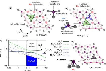
In Chapter 3, we explore the reconstructions of both Ni2P(0001) and Ni5P4(000±1)

surfaces with first principles DFT. Most of the stable terminations under realistic synthesis conditions are determined to be P-rich on both materials. A P-covered reconstruction of the Ni3P2 termination of Ni2P(0001) is found to be most stable,

consistent with the current literature. By contrast, the most energetically favorable surfaces of Ni5P4 are found to be the Ni3P3 and Ni4P3 bulk-derived terminations with

P-adatoms. The preferred excess P binding sites and their energies are identified on each surface. We find that the P3 site which is present on Ni5P4, and the Ni3 site,

which is present on both Ni2P and Ni5P4, strongly bind excess P. Additionally, we

predict the presence of stable Pn (n = 2,4) agglomerates on Ni5P4 at the P3-hollow

and Ni-Ni bridge sites. This chapter highlights the importance of considering the ag-gregation behavior of non-metal components in predicting the surface reconstruction of transition metal compounds. (67)

In Chapter 4, we explore, through DFT with thermodynamics, the aqueous re-constructions of Ni2P(0001) and Ni5P4(0001)/(000±1) and find that the surface P

content on Ni2P(0001) depends on the applied potential, which has not been

con-sidered previously. At -0.21 V ≥ U ≥ -0.36 V vs. the standard hydrogen electrode and pH = 0, a PHx-enriched Ni3P2 termination of Ni2P(0001) is found to be most

stable, consistent with its P-rich ultra-high-vacuum reconstructions. Above and be-low this potential range, the stoichiometric Ni3P2 surface is instead passivated by H

(34)

P. Instead, the Ni4P3 bulk termination of Ni5P4(000¯1) is passivated by H at both

the Ni3 and P3-hollow sites. We also found that the most HER-active surfaces are

Ni3P2+P+(7/3)H of Ni2P(0001) and Ni4P3+4H of Ni5P4(000¯1) due to weak H

ad-sorption at P catalytic sites, in contrast with other computational investigations that propose Ni as or part of the active site. By looking at viable catalytic cycles for HER on the stable reconstructed surfaces, and calculating the reaction free energies of the associated elementary steps, we calculate that the overpotential on the Ni4P3+4H

surface of Ni5P4(000¯1) (-0.16 V) is lower than that of the Ni3P2+P+(7/3)H surface

of Ni2P(0001) (-0.21 V). This is due to the abundance of P3-hollow sites on Ni5P4 and

the limited surface stability of the P-enriched Ni2P(0001) surface phase. The trend in

the calculated overpotentials explains why the nickel phosphides studied here perform almost as well as Pt, and why Ni5P4 is superior to Ni2P toward HER, as is found in

the experimental literature. This chapter emphasizes the importance of considering aqueous surface stability in predicting the HER-active sites, mechanism, and over-potential, and highlights the primary role of P in HER catalysis on transition metal phosphides. (38)

In Chapter 5, we investigate the effect of surface nonmetal doping on the HER activity of the Ni3P2 termination of Ni2P(0001), which is stable at modest

electro-chemical conditions. Using DFT calculations, we find that both 2p nonmetals and heavier chalcogens provide nearly thermoneutral H adsorption at moderate surface doping concentrations. We also find, however, that only chalcogen substitution for surface P is exergonic. For intermediate surface concentrations of S, the free en-ergy of H adsorption at the Ni3-hollow site is -0.11 eV, which is significantly more

(35)

charge descriptors, extracted from the DFT calculations, in determining the HER ac-tivity of Ni2P(0001) under different doping concentrations. We discover that the

Ni-Ni bond length is the most important descriptor of HER activity, which suggests that the nonmetal dopants induce a chemical pressure-like effect on the Ni3-hollow

site, changing its reactivity through compression and expansion. (39)

To overcome the limitations of ab initio thermodynamics and automate the dis-covery of realistic surfaces, we combine density functional theory and grand canonical Monte Carlo (GCMC) into “ab initio GCMC.” Chapter 6 presents the successful ap-plication of ab initio GCMC to the study of oxide overlayers on Ag(111), which, for many years, mystified experts in surface science and catalysis. Specifically, we report that ab initioGCMC is able to reproduce the surface phase diagram of Ag(111) with no preconceived notions about the system. Using nonlinear, random forest regres-sion, we discover that Ag coordination number with O and the surface O-Ag-O bond angles are good descriptors of the surface energy. Additionally, using the composition-structure evolution histories produced byab initioGCMC, we deduce a mechanism for the formation of oxide overlayers based on the Ag3O4 pyramid motif that is common

(36)

(a) Si(111)-7×7

(b) Au(110)-1×2

angle cavity

rest

atom _dimer adatom

faulted unfaulted

missing rows

top

side

(37)

CHAPTER 2 : Methodology

This thesis primarily consists of thermodynamic analyses of surface chemical reac-tions, namely surface reconstruction and heterogeneous catalysis. The thermody-namic properties of these processes, such as surface and adsorption free energies, can be readily computed given the total energies of the reactants and products and the forces acting on the atoms. The most accurate approaches for calculating total energies and forces are based on quantum mechanics. The quantum mechanical op-erator for the total energy is the Hamiltonian, which takes the following form for a polyatomic system ˆ H = N X I=1 − ~ 2

2MI ∇2

I+

X

I>J

ZIZJe2 |RI−RJ|

+ n X i=1 − ~ 2

2mi ∇2

i +

X

i>j e2

|ri−rj| − n X i=1 N X I=1

ZIe2 |ri−RI|

(2.1) where I/J and i/j are the nucleus and electron indices, N and n are the number of nuclei and electrons, _~ =h/2π is the reduced Planck constant, M and m are the nucleus and electron mass,∇2_{is the Laplace operator,}_Z _{is the nucleus charge in units}

of the electron chargee, andRandrare the positions of the nuclei and electrons. The first and second terms correspond to the kinetic energy and electrostatic repulsion of the nuclei, the third and fourth terms correspond to the kinetic energy ( ˆTee) and

electrostatic repulsion ( ˆVee) of the electrons (where ˆF = ˆTee+ ˆVee), and the fifth term

(38)

remains is to solve the electronic Schr¨odinger equation (70)

ˆ

HΨ (r;R) = Fˆ+ ˆVΨ (r;R) = E(R) Ψ (r;R) (2.2)

where Ψ is the electronic wave function and E is the total energy.

2.1. Density functional theory

One of the most powerful approaches to solve Eq. 2.2 is density functional theory (DFT). (71; 72) The key intuition of DFT is that the potential of the nuclei acts on only one electron at a time and therefore all one needs is the electron density to determine the potential energy. Based on this insight, we can write the potential as a sum over the potentials acting on each electron,i.e.

ˆ

V =X

i

V (ri) (2.3)

The expectation value of the potential is

hΨ

ˆ

V

Ψi=

Z

dr1· · ·drnΨ∗(r1,· · · ,rn) ˆVΨ (r1,· · · ,rn)

=X

j

Z

dr1· · ·drj· · ·drnΨ∗(r1, ...,rj, ...,rn)V (rj) Ψ (r1, ...,rj, ...,rn)

=X

j

Z

drjρj(rj)V (rj) =

Z

drρ(r)V (r)

(2.4)

(39)

2.1.1. Hohenberg-Kohn theorem

Using Eqs. 2.2 and 2.4, we can now prove the Hohenberg-Kohn (HK) theorem, which states that the potential is uniquely determined by the electron density. (71) Given two nondegenerate potentials ˆV1 and ˆV2, whose corresponding Ψ1 and Ψ2 are normalized,

we know from Eq. 2.2 that

E1 = Z

Ψ∗₁Fˆ+ ˆV1

Ψ1

E2 = Z

Ψ∗₂Fˆ+ ˆV2

Ψ2

(2.5)

where we have omitted differentials and position dependence for clarity. Additionally, we know from the variational principle that

Z

Ψ∗₁Fˆ+ ˆV2

Ψ1 > E2 Z

Ψ∗₂

ˆ

F + ˆV1

Ψ2 > E1

(2.6)

Inserting Eq. 2.5 into 2.6 and summing the two inequalities, we arrive at

Z

Ψ∗₁FˆΨ1+ Z

ρ1Vˆ2+ Z

Ψ∗₂FˆΨ2+ Z

ρ2Vˆ1 > Z

Ψ∗₁FˆΨ1+ Z

ρ1Vˆ1+ Z

Ψ∗₂FˆΨ2+ Z

ρ2Vˆ2

(2.7) If we assume that the potential is not uniquely determined by the electron density, in other words if ρ1 = ρ2, then Eq. 2.7 reduces to 0 > 0, which is clearly false,

(40)

2.1.2. Kohn-Sham equations

Having proven the HK theorem, we can write a total energy functional with the following general form

E[ρ(r)] =

Z

drV (r)ρ(r) +F [ρ(r)] (2.8)

whereF contains the electrostatic repulsion of the electrons, their kinetic energy, and exchange and correlation effects. In practice, electron-electron repulsion is included via classical electrostatics in the so-called “Hartree” energy

EH[ρ(r)] =

1 2

Z Z

drdr0ρ(r)ρ(r 0₎

|r−r0_| (2.9)

For the kinetic energy of the electrons, we introduce a set of noninteracting, single-electron “Kohn-Sham” wave functions {φi(r)} such that

TKS[ρ(r)] =

n X i=1 − ~ 2 2m Z

drφ∗_i (r)∇2φi(r) (2.10)

where

ρ(r) =

n

X

i

φ∗_i (r)φi(r) (2.11)

While the introduction of KS orbitals runs counter to the spirit of the HK theorem, state-of-the-art kinetic energy density functions tend to fail for materials with highly localized electron densities. (71; 73–75) Inserting Eqs. 2.9 and 2.10 into 2.8 yields

E[ρ(r)] =

Z

drV (r)ρ(r) + 1 2

Z Z

drdr0ρ(r)ρ(r 0₎

|r−r0_|

+ n X i=1 −~ 2 2m Z

drφ∗_i (r)∇2_φ

(41)

where Exc is the exchange-correlation energy, which contains electron exchange and

correlation effects as well as corrections for the self-interaction error (76) and the kinetic energy of interacting electrons. It is customary to rewrite the exchange-correlation functional as

Exc[ρ(r)] = Z

drxc[ρ(r)]ρ(r) (2.13)

In order to find the ground state total energy, we apply the variational principle by taking the functional derivative of Eq. 2.12 with respect to the KS orbitals

∂E[ρ(r)]

∂φ∗_i (r00₎ = 0 (2.14)

The first step in evaluating Eq. 2.14 is taking the derivative of the electron density

∂ρ(r)

∂φ∗_i (r00₎ =

∂ ∂φ∗_i (r00₎

n

X

j=1

φ∗_j(r)φj(r) = δ(r−r00)φi(r) (2.15)

Upon inserting Eqs. 2.12, 2.13, and 2.15 into 2.14 and integrating, we obtain

∂E[ρ(r)]

∂φ∗

i (r00)

=− ~

2

2m∇

2_φ

i(r00) +V (r00)φi(r00) +

Z

dr0 ρ(r 0₎

|r00₋_r0_|φ(r 00

)

+

∂xc(r00)

∂ρ(r00₎ ρ(r 00

) +xc(r00)

φ(r00)−λiφ(r00) = 0 (2.16)

where λ is a Lagrange multiplier that subjects the KS orbitals to an orthonormality constraint. Eq. 2.16 can be recast as

−~

2

2m∇

2₊_V ₍_r_{) +}_V

H(r) +Vxc(r)

(42)

where

VH(r) = Z

dr0 ρ(r 0₎

|r−r0_| (2.18)

is the Hartree potential and

Vxc(r) =

∂xc(r)

∂ρ(r) ρ(r) +xc(r) (2.19)

is the exchange-correlation potential. Eq. 2.17 is the familiar form of the KS equa-tions, which are traditionally solved using the following self-consistent procedure:

1. Specify positions of the nuclei {Ri} and calculate V (r)

2. Construct an initial guess for ρ(r), e.g.a superposition of atomic densities

3. Calculate VH(r) and Vxc(r)

4. Solve the KS equations numerically for {λi}and {φi(r)}

5. Construct the new ρ(r) from {φi(r)}

Steps 3-5 are repeated until the new and old electron densities are equal.

2.1.3. Local density approximation

(43)

exchange-correlation functional in Eq. 2.13, i.e.

E_xcLDA[ρ(r)] =

Z

drHEG_xc [ρ(r)]ρ(r) (2.20)

has proven quite successful. (79) Eq. 2.20 is known as the local density approximation (LDA). An intuitive reason for the success of the LDA is as follows. If you partition the electron density of a polyatomic system into infinitesimal volume elements, then, for each element, the density is nearly homogeneous. However, for systems with strongly spatially-varying electron densities, such as molecules, semiconductors, insulators, and crystals with defects, the LDA breaks down and more sophisticated exchange-correlation functionals are required.

2.1.4. Generalized gradient approximation

A natural extension of the LDA that favors density inhomogeneity is to include the gradient of the electron density in the exchange-correlation functional

E_xcGGA[ρ(r)] =

Z

drf[ρ(r),∇ρ(r)] (2.21)

This is called the generalized gradient approximation (GGA) and it has been shown to improve total energies, enthalpies of atomization, and activation energies for chemical reactions. (80–86) The most widely used GGA is that of Perdew, Burke, and Ernzerhof (PBE). (87) They proposed a correlation energy of the form

E_cGGA[ρ↑, ρ↓] =

Z

drρ

HEG_c (rs, ζ) +H(rs, ζ, t)

(2.22)

where we have omitted the position dependence of the electron density for clarity,

(44)

energy per electron of a homogeneous electron gas, rs = (3/4πρ)1/3 is the

Wigner-Seitz radius, that is, the radius of a sphere whose volume is equal to the volume per electron, ζ = (ρ↑−ρ↓)/ρis the relative spin polarization,t is a dimensionless density

gradient, and H is a gradient contribution that satisfies three conditions:

1. If ρ is slowly varying, i.e. as t→0, thenH ∝t2_{. (88)}

2. If ρ is fast varying, i.e. as t → ∞, then H ∝ −HEG

c . In other words, electron

correlation vanishes.

3. If ρ increases, i.e. asρ(r)→λ3_ρ₍_λ_r_{) and} _λ_{→ ∞}_{, then}_H _∝_ln_t2_{. (89)}

For more details on the construction of H, the reader is referred to the original paper. (87)

On the other hand, they define the exchange energy as

E_xGGA =

Z

drρHEG_x (ρ)Fx(s) (2.23)

where HEG

x = −3e2kF/4π is the exchange energy per electron of a homogeneous

electron gas, kF is the radius of the Fermi surface,s is another dimensionless density

gradient, and Fx is a gradient contribution that satisfies four additional conditions:

1. Ex[ρ↑, ρ↓] = (Ex[2ρ↑] +Ex[2ρ↓])/2. (90)

2. If ρ=ρHEG_, _i.e. _if _s_{= 0, then} _F x= 1.

3. If ρis slowly varying, then the LDA is a better approximation for the exchange-correlation energy than the GGA. (91–93) Therefore, as s → 0, Fx ∝ 1 +

(45)

4. Ex[ρ↑, ρ↓]≥Exc[ρ↑, ρ↓]. (94)

This thesis comprises DFT calculations performed using the GGA of PBE.

2.1.5. Bloch’s theorem and the plane wave basis set

In order to solve the KS equations numerically, we must choose a computational representation of the KS orbitals. This usually amounts to choosing a set of basis functions in which to expand the KS orbitals. A particularly fortuitous choice is a basis set consisting of plane waves, for reasons that will now be explained. In this thesis, we are primarily concerned with crystals and models of their surfaces that are periodic in three dimensions. When modeling a solid material with periodicity, it becomes unnecessary to consider the infinite number of atoms and electrons present in the macroscopic crystal. Instead, due to the underlying symmetry of the crystal, one can often identify a relatively small, fundamental repeating unit known as a primitive cell. Bloch’s theorem states that we can use this periodicity to express the electronic wave function as

φnk(r) = eik·runk(r) (2.24)

where we have replaced i with n as the index of the energy band to avoid confusion with the imaginary numberi,kis a wave vector, andunk(r) is a function that has the

same periodicity as the crystal, i.e. unk(r) = unk(r+L) where L is a translational

vector of the primitive cell. (95) Plane waves are a natural choice to expand unk(r)

because they form a complete and orthonormal basis and can be made to satisfy the periodic boundary conditions of the crystal

(46)

whereG is a reciprocal lattice vector andG·L= 2π×integer. Expanding unk(r) in

plane waves,

unk(r) = X

G

cnk(G)eiG·r (2.26)

where cnk are coefficients that depend on G, and inserting Eq. 2.26 into 2.24 gives

φnk(r) = X

G

cnk(G)ei(k+G)·r (2.27)

Substitution of Eq. 2.27 into the KS equations (2.17) and integration overrproduces

X

G0

~2

2m|k+G|

2

δGG0 +V (G−G0) +V_H(G−G0) +V_xc(G−G0)

cnk(G0)

=λncnk(G) (2.28)

where V, VH, and Vxc are described in terms of their Fourier transforms. At this

point, we will briefly discuss some technical aspects related to the sum over G0 and the selection of k. In principle, Eq. 2.28 contains an infinite sum over G0 because there is an infinite number of repeats of the primitive cell in a macroscopic crystal. Of course, one can always choose to truncate this sum to make Eq. 2.28 computationally tractable. Typically, this is done in a systematic way by placing a cutoff on the kinetic energy of the plane waves included in the expansion, that is to say, the kinetic energy of a plane wave whose wave vector isk+Gmust be less than some energy cutoff Ecut

Ek+G= ~

2

2m|k+G|

2

< Ecut (2.29)

whereEcut can be increased to achieve higher levels of total energy and force

(47)

energy of the system. As for the selection ofk, the exact solution of the KS equations involves an integral over the Brillouin zone. However, like the infinite sum over G0, this too is impossible. It has been shown that the integral overkcan be replaced by a sum over a finite set of k-points also known as a k-point mesh. (96; 97) For practical DFT calculations, one usually benchmarks the convergence of the total energy and forces against the density of the k-point mesh.

2.1.6. Pseudopotentials

Once the KS equations have been written in a plane wave basis, they can be solved by diagonalizing the matrix whose elements are given by Eq. 2.28. As the size of the system increases, however, so does the size of this matrix thus making the solution of the KS equations prohibitively expensive for all but the smallest systems containing elements with the fewest electrons. This scaling can be improved by recognizing the fact that the chemical bonding in a crystal is dominated by the valence electrons of the constituent atoms. (98–102) Another complication is that the wave functions of the valence electrons oscillate rapidly near the core, which increases the number of plane waves required for their description. To overcome these limitations, we can replace the hard ionic potential with a soft, effective potential that includes the interactions between the nucleus and core electrons and reproduces the eigenvalues and tails of the all-electron valence wave functions (see Fig. 2.1 for a P pseudopotential). This replacement is known as the pseudopotential approximation and it frequently accom-panies the use of a plane wave basis. The first step of pseudopotential construction is to solve the radial KS equations for the all-electron (AE) eigenvalues {λAE

l } and

wave functions {φAE

l (r)} of a reference atomic electron configuration

− d

2

dr2 +

l(l+ 1)

r2 −

2Z

r +VHxc[ρ(r)]

(48)

where l is the orbital angular momentum quantum number and VHxc = VH +Vxc.

Next, pseudo-wave functions (PS) are designed such that the following five rules are upheld:

1. {λAE

l }ref ={λPSl }ref.

2. φAE_l,_ref =φPS_l,_ref for r ≥rc whererc is a user-defined cutoff radius.

3. N_l,AE_ref =N_l,PS_ref whereNl=Rrc

0 drr

2_|φl₍_r₎_|2

.

4. DAE

l (λ, rc) = DlPS(λ, rc) where Dl(λ, rc) = r_drd lnφl(λ, rc).

5. _∂λ∂ DAE

l (λ, rc) = _∂λ∂ DPSl (λ, rc).

If a pseudo-wave function obeys rules 3 and 5, then the resulting pseudopotentials are called “norm-conserving”. (103) Once the pseudo-wave functions have been designed, screened (scr) semi-local pseudopotentials are calculated by inverting Eq. 2.30, which yields

V_lscr(r) = λl−

l(l+ 1)

r2 +

1

φPS

l (r) d2

dr2φ PS

l (r) (2.31)

The screened pseudopotentials are then descreened to give the ionic pseudopotentials

V_lPS(r) =V_lscr(r)−VHxc

ρval(r) (2.32)

where ρval(r) is the valence electron density. The ionic pseudopotentials of P are shown at the bottom of Fig. 2.1. Eq. 2.32 suggests that each orbital angular momen-tum of the wave function experiences a different ionic potential.

(49)

fully separable, nonlocal (NL) form

ˆ

VNL =Vloc(r) + X

l

∆V_l(r)φ_lref φref_l ∆V_l(r) φref l

∆Vl(r)

φref_l

(2.33)

where Vloc(r) is an arbitrarily chosen local potential and

∆Vl(r) =VlPS(r)−Vloc(r) (2.34)

This is the well-known Kleinman-Bylander nonlocal form. (104) Further, it has been shown that the transferability of a nonlocal pseudopotential,i.e. its ability to repro-duce all-electron calculations of non-reference states, can be enhanced by adding an augmentation functionA(r) to the local potential

ˆ

VDNL =Vloc(r) +A(r) + X

l

(∆Vl(r)−A(r))φ_lref φref_l (∆Vl(r)−A(r)) φref l

(∆V_l(r)−A(r)) φref_l

(2.35)

(50)

0.0 0.5 1.0 1.5 2.0 2.5 r(Å) 0.4 0.2 0.0 0.2 0.4 0.6 0.8 r ( r ) AE 3s AE 3p AE 3d NL 3s NL 3p NL 3d

0.0 0.5 1.0 1.5 2.0 2.5

r(Å) 400 200 0 200 400 600 Vion (eV)

V3s V3p V3d 2Zeff/r

Vloc

Figure 2.1: Pseudopotential of P. (Top) All-electron (AE) wave functions and non-local (NL) pseudo-wave functions of the P 3s, 3p, and 3d states. NL pseudo-wave functions are nodeless and smoother than the AE wave functions. (Bottom) Ionic pseudopotentials V3l, true atomic potential (shaded red), and local potential Vloc.

(51)

2.1.7. van der Waals interactions

A drawback of the LDA and GGA is that the resulting exchange-correlation function-als are unable to correctly describe the nonlocal electron correlations responsible for van der Waals (vdW) interactions. (107; 108) For example, GGAs tend to underesti-mate their strength. (109; 110) This is of great concern because vdW interactions can influence the thermodynamics of chemical reactions, which is the central topic of this thesis. (111–119) In order to rectify the GGA’s treatment of vdW interactions, many different corrections have been proposed. (120–128) Of those, perhaps the simplest is the semiempirical correction of the form

EvdW =−

1 2

N

X

i=1

N

X

j=1 X

L C6ij r6

ij,L

fd,6(rij,L) (2.36)

where C6ij are the vdW coefficients of the atom pair ij, rij,L is the distance between

atomiin the primitive cell and atomj in a neighboring cell translated from the origin by L, and fd,6 is a damping function that avoids the counting of vdW interactions

between atoms at chemical bonding distances. (129) The vdW coefficients of atom pairs can be written as the geometric mean of atomic vdW coefficients

C6ij =

q

Ci

6C

j

6 (2.37)

where C6 of atom i is given by

C₆i = 0.05×mI_piαi_p (2.38)

(52)

quantum mechanical foundation as it is derived from the London formula. (130–132) The form of the damping function is flexible, however, it is typically expressed as

fd,6(rij) =

s6

1 +e−d(rij/R0ij−1) (2.39)

where s6 is a scaling factor that depends on the exchange-correlation functional,d is

a damping parameter, and R0ij is

R0ij =Ri0+R

j

0 (2.40)

where Ri

0 is the vdW radius of atom i. (129) To apply this vdW correction, Eq. 2.36

is simply added to the KS total energy. The forces, on the other hand, are computed from finite differences.

2.2. Ab initio

thermodynamics

The primary goal of this thesis is to determine the thermodynamic barriers associated with surface chemical reactions, specifically those occurring in an electrochemical environment. Such an endeavor requires knowledge of the Gibbs free energies of the reactants, products, and intermediate species in the chemical reaction of interest. The Gibbs free energyGis the Legendre transform of the internal energyU(S, V, N), which results in

G=U −T S+pV (2.41)

dG=−SdT +V dp+µdN (2.42)

(53)

is the differential form of G for a quasistatic process. G(T, p, N) is an example of a thermodynamic potential, which is a scalar that represents the state of a thermody-namic system. It describes the capacity of a system to do non-mechanical work and is minimized, in other words,dG= 0, when the system reaches chemical equilibrium at constantT andp. It follows from this thatGmust decrease for a chemical reaction to be spontaneous.

For reasons that will soon be evident, it is important to know the relationship between µ, T, and p. µ is defined as

µ= ∂G ∂N T ,p (2.43)

Multiplying both sides of Eq. 2.43 bydN and integrating, we find thatGand dGcan be expressed as

G=µN =

I

X

i=1

µiNi (2.44)

dG=

I

X

i=1

µidNi+ I

X

i=1

Nidµi (2.45)

where the sum is over the types of particles, of which there are I. By setting Eqs. 2.42 and 2.45 equal, we obtain

I

X

i=1

Nidµi =−SdT +V dp (2.46)

(54)

First, let us consider the isothermal compression/expansion of an ideal gas. This is relevant to our study of surface chemical reactions because the reactants/products may be in the gas phase and, under certain circumstances, behave like ideal gases. For constant T, Eq. 2.46 becomes

N dµ=V dp (2.47)

for a single phase ideal gas. Replacing V in Eq. 2.47 with the ideal gas equation of state and integrating yields

∆µ=kBT ln

pf pi

(2.48)

wherekB is the Boltzmann constant, andpf andpi are the final and initial pressures,

respectively.

Since we are interested in the chemical reactivity of crystals, we should also consider the isothermal compression/expansion of solids. Unfortunately, solids do not have a simple equation of state like ideal gases. Progress can be made in deriving ∆µ, however, by noting that the isothermal compressibility of solids is small, i.e.

βT =−1 V

∂V ∂p

T

≈0 (2.49)

From Eq. 2.49, it is clear that the volume is constant with respect to quasistatic changes in pressure. Using this result, we integrate Eq. 2.47

∆µ= 1

N

Z

V dp= 1

ρ(pf −pi) (2.50)

(55)

to the free energy changes of chemical reactions and therefore can be safely neglected.

Now, let us consider the isobaric heating/cooling of a system. For constantp, the integrated form of Eq. 2.46 is

∆µ=−1 N

Z

SdT (2.51)

We do not know, however, an equation of state that relatesS andT. Another way to approach this problem is to start with the thermodynamic potential that corresponds to constant p, i.e. the enthalpy

H =U +pV (2.52)

dH =T dS+V dp+µdN (2.53)

For an isobaric process,

∆H =

Z

T dS =

Z

cpdT (2.54)

where we have replaced T dS with the definition of the isobaric heat capacity

cp =T

∂S ∂T

p

(2.55)

∆H in Eq. 2.54 is called the integrated heat capacity (IHC). Combining Eqs. 2.41, 2.44, 2.52, and 2.54, one obtains

∆µ= 1

N

Z

cpdT −∆ (T S)

(2.56)

(56)

We are now ready to calculate the free energy changes of chemical reactions. Consider the general chemical reaction

NR

X

i=1

miRi NP

X

j=1

njPj (2.57)

where NR and NP are the number of reactants (R) and products (P), i and j are

their indices, andm and n are their stoichiometric coefficients, respectively. The free energy change of this reaction (rxn) is

∆Grxn =

NP

X

j=1

njGj − NR

X

i=1

miGi

=

NP

X

j=1

njHj − NP

X

j=1

njT Sj+ NP

X

j=1

njIHCj(T)

− NR

X

i=1

miHi+ NR

X

i=1

miT Si− NR

X

i=1

miIHCi(T)

= ∆Hrxn−T∆Srxn+ ∆IHCrxn(T)

(2.58)

where ∆Hrxn is the enthalpy change and ∆IHCrxn is the integrated heat capacity

change. Practically speaking, H is approximated by the DFT total energy, which corresponds to 0 K. S and the IHC are taken from thermochemical tables. (133; 134)

For surface chemical reactions, the free energy changes associated with the vi-brations of surface atoms and adsorbates must also be taken into account. To un-derstand why this is necessary, consider the following example. In the gas phase, H2 has a stretching frequency of 4401 cm−1. (135) On the Pt(111) surface, however,

(57)

small but nonzero and therefore important for obtaining quantitative agreement with experiments. We start from the partition function Z of a harmonic solid

Z =

3N

Y

i=1

e−~ωi/2kBT

1−e−~ωi/2kBT (2.59)

where ωi is the vibrational frequency of oscillator i. Z is related to the vibrational

free energy via

Fvib =−kBTlnZ =

1 2

3N

X

i=1

~ωi+kBT 3N

X

i=1

ln 1−e−~ωi/kBT _(2.60)

where the first sum on the right-hand side is the zero-point energy (ZPE). At high temperatures, the harmonic approximation breaks down because the atomic vibra-tions can now sample regions of the potential energy surface where anharmonic effects are important. Therefore, one must be careful, when using Eq. 2.60, to ensure that the system is in the harmonic regime at the temperatures of interest. Here, ωi were

calculated using density-functional perturbation theory (DFPT). (137)

2.2.1. Bulk phase diagrams

Before we can study chemical reactions on a surface, we first have to determine the conditions under which the bulk crystal is stable. This is done by constructing a bulk phase diagram, which plots the thermodynamically preferred bulk phase as a function of the chemical potentials of the constituent elements. Take, for example, the hypothetical binary compound AxBy, which has three stable chemical compositions, x1/y1 < x2/y2 < x3/y3. The chemical equilibrium of Ax2By2 is

(58)

The free energy of Ax2By2 formation can be written as

∆Gf,Ax₂By₂ =x2∆µA+y2∆µB (2.62)

Here, ∆µ =µ−Estd where Estd is the DFT total energy of the standard state. Eq.

2.62 shows that the equilibrium in Eq. 2.61 is a line in the (∆µA, ∆µB) plane. If

one phase occurs on a line, then two phases coexist at the point where their lines intersect. The coordinates of the intersection of Ax1By1 and Ax2By2 is calculated by

solving the following matrix equation



 

x1 y1

x2 y2 

 



 

∆µA

∆µB 

 =



 

∆Gf,Ax₁By₂

∆Gf,Ax₂By₂





 (2.63)

C∆~µ=∆~Gf (2.64) ~

∆µ=C−1∆~Gf (2.65)

The same procedure is repeated for the equilibrium between Ax2By2 and Ax3By3. The

resulting sets of chemical potentials,∆~µ₁₂ and∆~µ₂₃, enclose the region where Ax2By2

(59)

5

4

3

2

1

0

A

5

4

3

2

1

0

B

min

B

max

B

m

in

A

m

ax

A

AB is stable

A

2

B

AB

2

Figure 2.2: Bulk phase diagram of a hypothetical binary compound AxBy with three

stable compositions A2B, AB, and AB2. Dotted lines enclose the region of ∆µA and

Toward Realistic Modeling Of Catalytic Surfaces: From First Principles To Machine Learning

ScholarlyCommons

ScholarlyCommons

Toward Realistic Modeling Of Catalytic Surfaces: From First

Toward Realistic Modeling Of Catalytic Surfaces: From First

Principles To Machine Learning

Principles To Machine Learning

Toward Realistic Modeling Of Catalytic Surfaces: From First Principles To

Toward Realistic Modeling Of Catalytic Surfaces: From First Principles To

Machine Learning

Machine Learning

ACKNOWLEDGEMENTS

ABSTRACT

TABLE OF CONTENTS

LIST OF TABLES

LIST OF ILLUSTRATIONS

PREFACE

CHAPTER 1 : Introduction

(a) Si(111)-7×7

(b) Au(110)-1×2

CHAPTER 2 : Methodology

2.1. Density functional theory

2.2.

Ab initio

thermodynamics

5

4

3

2

1

0

5

4

3

2

1

0

min

max

m

in

m

ax

AB is stable

A

B

AB

AB