RELIABILITY IMPROVEMENT OF
RADIAL DISTRIBUTION SYSTEM
WITH DISTRIBUTED GENERATION
G.V.K MURTHY,
Associate Professor, Dept. of EEE, SSNEC, Ongole, A.P., INDIA.
Dr. S.SIVANAGARAJU,
Associate Professor and Head, Dept. of EEE, JNTUK, Kakinada, AP, INDIA.
Dr. S.SATYANARAYANA,
Principal,
VRSYRN CET, Chirala, AP, INDIA. [email protected]
B. HANUMANTHA RAO,
Dept. of EEE, UCE, JNTUK, Kakinada, AP, INDIA.
Abstract— This paper describes a methodology for reliability enhancement of radial distribution system with Distributed Generation (DG). Assessment of customer power supply reliability is an important part of distribution system operation and planning. Distribution system reliability assessment is able to predict the interruption profile of a distribution system based on system topology and component reliability data. Distributed generation is being adopted in distribution networks with one of the objectives being enhancement of system reliability. Artificial Bee Colony (ABC) algorithm is proposed to obtain the optimal values of repair times and failure rates of each section to improve the reliability.
Key words – distributed generation, artificial bee colony algorithm, reliability indices, failure rate, repair time, radial distribution network.
I. INTRODUCTION
The majority of distribution systems are designed to operate with a radial topology. Radial distribution systems have a set of series components between a substation and a load point, including breakers, lines, cables, transformers, switches, fuses and other equipment. A failure of any component in the series path results in the outage of a load point. Sectionalizing devices provide a means of isolating a faulted section. In some systems there is an alternative supply source for sections that become disconnected from their original source after the failure is isolated.
Distribution reliability primarily relates to equipment outages and customer interruptions. In normal operating conditions, all equipments (except standby) are energized and all customers are energized. Scheduled and unscheduled events disrupt normal operating conditions and can lead to outages and interruptions. A reliability assessment model quantifies reliability characteristics based on system topology and component reliability data. Areas of inherently good or poor reliability can be identified. The model also identifies over-loaded and undersized equipment that degrades system reliability. Other useful results include the expected number of switch and protective device operations and the sensitivity of results to component reliability parameters.
DG may be high. Further the traditional reliability indices covered sustained interruption durations. The time necessary to start up the DG should be taken in to account for the reliability evaluation of distribution system. If this time is sufficiently short the customers suffer a momentary interruption, while, if not, they suffer a sustained interruption.
Distributed generation (DG) is expected to play an increasing role in emerging power systems [1]. Studies have predicted that DG will be a significant percentage of all new generation going online. Different resources can be used in DG. Its impact on distribution systems may be either positive or negative depending on the system’s operating condition [1-2], DGs characteristics and location. Potential positive impacts include
improved system reliability; loss reduction;
improved power quality.
Two sets of reliability indices, customer load point indices and system indices have been established to assess the reliability performance of distribution systems. Load point indices measure the expected number of outages and their duration for individual customers. System indices such as System Average Interruption Duration Index (SAIDI) and System Average Interruption Frequency Index (SAIFI) measure the overall reliability of the system [3]. These indices can be used to compare the effects of various design and maintenance strategies on system reliability.
Optimal allocation and sizing of DGs is solved in [4] using an analytical based method to minimize the line loss. The same problem is solved using an ordinal optimization method in [5]. In addition to the line loss, the system reliability is included in the DG planning problem as a constraint in [6] for improving the system reliability, line loss, and voltage profile. In [6], the genetic algorithm (GA) is employed as the required optimization method.
To further improve the system reliability, switches, such as reclosers and cross connections, are incorporated in the DG-based planning problem. An ant colony system algorithm is employed in [7] for finding the optimal placement of reclosers and DGs. This method minimizes an objective function composed of two reliability indices: system average interruption duration index and system average interruption frequency index. A two-step design is presented in this paper. First, the optimal placement of reclosers is identified while the DG locations are fixed. Then, DGs are planned for the reclosers determined in the previous step. A similar problem with the same objective function is solved using GA in [8] and [9]. In [10], an ant colony algorithm based reconfiguration methodology is proposed for solving the optimal switching operation of distribution networks in the presence of DGs.
This paper presents artificial bee colony (ABC) method for optimal failure rate and repair time of each section of a distribution system in the presence of distributed generation. An objective function which reflects cost of modification of failure rates, and repair rate and cost of energy not supplied from DG has been constructed and minimized subject to reliability constraints.
II. PROBLEM FORMULATION
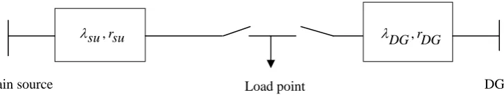
Distributed generation may be used as standby units for reliability enhancement at specific load points. If DG capacity is sufficient to meet the load at a load point in the event of failure of supply from substation then the situation at load point is represent as shown in Fig. 1.
Fig 1. Load point fed from main source and DG as stand by unit
Where,
su
is the total failure rate up to load point from source,
rsu is the average interruption duration from source,
DG
is the failure rate of DG, ,r
su su
DG DG,r
rDG is the average outage duration of DG.
Reliability may be improved for a radial distribution system by modifying failure rate and average repair time of each segment of the system. Addition of distribution generation (DG) may require additional cost per kWh to be paid to the private DG owners. In view of this the objective function is selected as follows
1 1
2
1 1
n k n k
F ADCOST EENSO EENSD
k k rk k
(1)
Where
k
is the failure rate of kth section, rk is the average repair time of kth section,
αkand βk are the cost coefficients,
EENSO is the expected energy not supplied without DG,
EENSD is the expected energy not supplied with DG.
The objective function constitutes of three parts i.e. first part reflects cost of modifications of failure rates of each section, second part gives cost of modifications in average repair time of each section which is again based on a growth model of repair time and third part represents additional cost to be paid to the owners of DG. This term in fact is the expected energy supplied (EENSO–EENSD) by DG multiplied by additional charge per kWh (ADCOST).
Expected energy not supplied (EENS) is calculated for all load points as follows
, EENS L Ui system i
i
(2)
Where Liis average load at ith load point; USystem,i is average annual outage duration at ith load point. EENS is calculated without DG is termed as EENSO and that calculated with DG is termed as EENSD.
Calculate Usustem,i accounting without DG to evaluate EENSO as follows
,
Usystem i k kr k d
‘d’ is set of distribution segments in series up to kth load point. Calculate Usustem,i accounting with DG to evaluate EENSD as follows
,
Usystem i eq eqr
eq st
req s
Where λst is the failure rate of manual switch
‘s’ is average time to carry out the switching operation.
The objective function is minimized subject to following customer and energy based constraints
1. System average interruption frequency index,
λ N
Total number of customers interruptions system, i i
SAIFI = =
Total number of customers served Ni
(3)
Where Ni is the number of customers at load point ‘i
2. System average interruption frequency index,
U N
Sum of customer interruptions durations system,i i
SAIDI = =
Total number of customers served Ni
3. Customer average interruption duration index,
U N
Sum of customer interruption durations system, i i
CAIDI = =
Total number of customer interruptions Ni system, iλ
(5)
4. Average service availability index,
N × 8760 - N U
Customer hours of available service i i system, i
ASAI = =
Customer hours demanded N × 8760i
(6)
5. Average service interruption duration index,
r L Connected kVA duration interrupted i i
ASIDI = =
Total connected kVA served LT (7)
Where Li is average load connected to load point ‘i’
6. Average service interruption frequency index,
L Connected kVA interrupted i
ASIFI = =
Total connected kVA served LT
(8)
7. Average customer interruption duration index,
r L Connected kVA duration interrupted i i
ACIDI = =
Connected kVA interrupted Li
(9)
8. Average energy not supplied indices,
L U Total energy not supplied i i
AENS = =
Total number of customers served Ni
(10)
III. ARTIFICIAL BEE COLONY ALGORITHM (ABC)
Artificial Bee Colony (ABC) is one of the most recently defined algorithms by Dervis Karaboga in 2005, motivated by the intelligent behavior of honeybees. ABC as an optimization tool provides a population based search procedure in which individuals called food positions are modified by the artificial bees with time and the bee’s aim is to discover the places of food sources with high nectar amount and finally the one with the highest nectar. In this algorithm [11, 12], the colony of artificial bees consists of three groups of bees: employed bees, onlookers and scouts. First half of the colony consists of the employed artificial bees and the second half includes the onlookers. For every food source, there is only one employed bee. In other words, the number of employed bees is equal to the number of food sources around the hive. The employed bee whose food source has been abandoned becomes a scout [13].
Thus, ABC system combines local search carried out by employed and onlooker bees, and global search managed by onlookers and scouts, attempting to balance exploration and exploitation process [14].
The ABC algorithm creates a randomly distributed initial population of solutions (f = 1,2,…..,Eb),
where ‘f’ signifies the size of population and ‘Eb’ is the number of employed bees. Each solution xf is a
taken from all employed bees and chooses a food source with a probability related to its nectar amount. The same procedure of position modification and selection criterion used by the employed bees is applied to onlooker bees. The greedy-selection process is suitable for unconstrained optimization problems. The probability of selecting a food-source pf by onlooker bees is calculated as follows:
fitness P =
f E b
fitnessf f =1
(11)
Where fitnessf is the fitness value of a solution f , and Eb is the total number of food-source positions
(solutions) or, in other words, half of the colony size. Clearly, resulting from using (11), a good food source (solution) will attract more onlooker bees than a bad one. Subsequent to onlookers selecting their preferred food-source, they produce a neighbor food-source position f+1 to the selected onef, and compare the nectar amount (fitness value) of that neighbor f+1 position with the old position. The same selection criterion used by the employed bees is applied to onlooker bees as well. This sequence is repeated until all onlookers are distributed. Furthermore, if a solution f does not improve for a specified number of times (limit), the employed bee associated with this solution abandons it, and she becomes a scout and searches for a new random food-source position. Once the new position is determined, another ABC algorithm (MCN) cycle starts. The same procedures are repeated until the stopping criteria are met.
In order to determine a neighboring food-source position (solution) to the old one in memory, the ABC algorithm alters one randomly chosen parameter and keeps the remaining parameters unchanged. In other words, by adding to the current chosen parameter value the product of the uniform variant [-1, 1] and the difference between the chosen parameter value and other “random” solution parameter value, the neighbor food-source position is created. The following expression verifies that:
new old old
xfg = xfg + u xfg - xmg (12)
Where m f and both are
1, 2, ..., E
b . The multiplier u is a random number between [-1, 1] and
g 1, 2, ..., D . In other words, xfg is the gth parameter of a solution xf that was selected to be modified. When
the food-source position has been abandoned, the employed bee associated with it becomes a scout. The scout produces a completely new food source position as follows:
new
xfg = min xfg + u max x
fg - min xfg
(13)Where (13) applies to all g parameters and u is a random number between [-1, 1]. If a parameter value produced using (12) and/or (13) exceeds its predetermined limit, the parameter can be set to an acceptable value. In this paper, the value of the parameter exceeding its limit is forced to the nearest (discrete) boundary limit value associated with it. Furthermore, the random multiplier number u is set to be between [0, 1] instead of [-1, 1].
Thus, the ABC algorithm has the following control parameters: 1) the colony size CS, that consists of employed bees Eb plus onlooker bees Eb ; 2) the limit value, which is the number of trials for a food-source
position (solution) to be abandoned; and 3) the maximum cycle number MCN .
The proposed ABC algorithm is as follows:
Step-1: Initialize the food-source positions xf (solutions population), where f = 1,2,…..,Eb. The xf solution form
is as follows.
Step-2: Calculate the nectar amount of the population by means of their fitness values using equation (1)
Step-3: Produce neighbor solutions for the employed bees by using (12) and evaluate them as indicated by Step 2.
Step-4: Apply the greedy selection process.
Step-7: Produce neighbor solutions for the selected onlooker bee, depending on the value, using equation (1) and evaluate them as Step 2 indicates.
Step-8: Follow Step 4.
Step-9: Determine the abandoned solution for the scout bees, if it exists, and replace it with a completely new solution using (13) and evaluate them as indicated in Step 2.
Step-10: Memorize the best solution attained so far.
Step-11: If cycle = MCN, stop and print result. Otherwise follow Step 3.
IV. RESULTS AND ANALYSIS
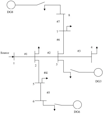
The proposed method is tested on 8-bus distribution system as shown in Fig 2. The system has been modified due to presence of DG at bus-3, bus-6 and bus-8. In the failure of supply from the source at these nodes continuity is maintained with the help of these distributed generations. The data of failure rates, repair time, average load, number of customers and cost coefficients are given in [15]. The ADCOST is selected as Rs.1.5 per kWh in the objective function.
Fig 2. 8- Bus radial distribution system with DG at selected load points
Reliability modeling aspects for load points are calculated as follows
λsystem,2=λ1
rsystem,2= r1
Usystem,2=λ1 1r Source
1
DG3
2 3
4
5
6
7
8
DG6 DG8
#5
#4
#1 #2 #3
λsystem,4=λ1+λ2+λ3
Usystem,4=λ1 1r +λ2 2r +λ3 3r
U system,4
rsystem,4=
λsystem,4
λsystem,5=λ1+λ4
Usystem,5=λ1 1r +λ4 4r
U system,5
rsystem,5=
λsystem,5
λsystem,7=λ1+λ2+λ6
Usystem,7=λ1 1r +λ2 2r +λ6 6r
U system,7
rsystem,7=
λsystem,7
The distributed generations are present at buses 3, 6 and 8. The calculation of basic reliability indices will be different as follows
λsystem,3=λst3
λsystem,3=λst3
Where λst3 is the failure rate of manual switch of DG3
rsystem,3= s3
Where s3 is average service restoration time of DG3
Usystem,3=λst3 3s
Similarly, The basic reliability indices of DG6 and DG8 as follows
λsystem,6=λst6,rsystem,6= s6,Usystem,6=λst6 6s and λsystem,8=λst8
rsystem,8= s8, Usystem,8=λst8 8s
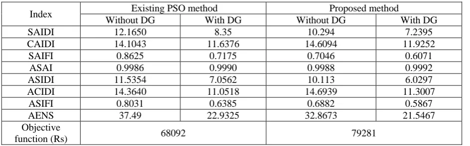
Table 1: The optimum values of failure rate and repair time
Distribution section Variables
Existing PSO method
Proposed
method Variables
Existing PSO method
Proposed method Failure rates (Year) Repair times (Hours)
1 λ1 0.6 0.6 r1 15 15
2 λ2 0.3 0.05 r2 14 7.5529
3 λ3 0.1 0.1 r3 4 4
4 λ4 0.1 0.1 r4 8 27.0991
5 λ5 0.15 0.2213 r5 22 7
6 λ6 0.15 0.0583 r6 6 11.3771
7 λ7 0.05 0.05 r7 6 6
Reliability indices for 8-bus radial distribution system are given in Table 2. From the Table 2 the system average interruption duration index (SAIDI) of the system is 10.294 without DG and 7.2395 with DG by ABC method. Note that the decrease of SAIDI indicates an increase of the system reliability. Because of SAIDI depends upon failure rate and repair time of the equipment.
Table 2: Reliability indices for radial distribution system
Index Existing PSO method Proposed method
Without DG With DG Without DG With DG
SAIDI 12.1650 8.35 10.294 7.2395
CAIDI 14.1043 11.6376 14.6094 11.9252
SAIFI 0.8625 0.7175 0.7046 0.6071
ASAI 0.9986 0.9990 0.9988 0.9992
ASIDI 11.5354 7.0562 10.113 6.0297
ACIDI 14.3640 11.0518 14.6939 11.3007
ASIFI 0.8031 0.6385 0.6882 0.5867
AENS 37.49 22.9325 32.8673 21.5467 Objective
function (Rs) 68092 79281
SAIDI of the system is 8.35 with DG by PSO method and 7.2395 with DG by ABC method. It can be observed the duration related indices improvement with DG installation. Similarly other reliability indices CAIDI, SAIFI, ASIDI, ACIDI, ASIFI and AENS are reduced with DG except ASAI. Average service availability index (ASAI) is improved from 0.9988 to 0.9992 with distributed generations. It can also be seen that the objective function given by the ABC method is 79281 and 68092 by PSO method. It is observed that the objective function obtained by the proposed method is greater than the existing PSO method.
V. CONCLUSION
The reliability improvement is important effect of DGs in emerging active distribution networks. Reliability is measured by reliability indices SAIDI, ASAI, CAIDI, SAIFI, ASIDI, ACIDI, ASIFI and AENS. Electrical power distribution reliability can be improved from different aspects, from planning to operation and maintenance. This paper presents reliability improvement of radial distribution system in the presence of distributed generation. An optimization problem has been formulated which obtains optimum failure rates and repair times of each section. The proposed ABC method is effective as compared to PSO method in terms of objective function improvement.
VI. REFERENCES
[1] P. P Barker. and R. W. De Mello, “Determining the impact of distributed generation on power systems: Part 1- Radial distribution systems,” IEEE Power technology, Inc, Vol. 3, pp. 1645–1656, 2000.
[2] R. E. Brown and L. A. A. Freeman, “Analyzing the reliability impact of distributed generation,” IEEE, Power Engineering Society. Summer Meeting, Vol. 2, pp. 1013–1018, 2001.
[3] IEEE Trial Use Guide for Electric Power Distribution Reliability Indices, IEEE Std. 1366-1998, 1999.
[4] T. Gozel and M. H. Hocaoglu, “An analytical method for the sizing and siting of distributed generators in radial systems,” Electric Power System, Vol. 79, pp. 912–918, 2009.
[5] R. A. Jabr and B. C. Pal, “Ordinal optimization approach for locating and sizing of distributed generation,” IET Generation, Transmission & Distribution, Vol. 3, pp. 713–723, 2009.
[7] L. Wang and C. Singh, “Reliability constrained optimum placement of reclosers and distributed generators in distribution networks using an ant colony system algorithm,” IEEE Transaction on systems and Mantainance, Vol. 38, pp. 757–764, 2008.
[8] A. Pregelj, M. Begovic, and A. Rohatgi, “Recloser allocation for improved reliability of DG enhanced distribution networks,” IEEE Transaction on Power System, Vol. 20, pp. 1442–1449, 2006.
[9] D. H. Popovic, J. A. Greatbanks, M. Begovic, and A. Pregelj, “Placement of distributed generators and reclosers for distribution network security and reliability,” International journal of electrical power energy systems, Vol. 27, pp. 398–408, 2005.
[10] Y. K. Wu, C. Y. Lee, L. C. Liu, and S. H. Tsai, “Study of reconfiguration for distribution system with distributed generators,” IEEE Transaction on power delivery, Vol. 25, pp. 1678–1685, 2010.
[11] Dervis Karaboga and Bahriye Basturk, “Artificial Bee Colony (ABC) Optimization Algorithm for Solving Constrained Optimization Problems,” Springer-Verlag, IFSA 2007, LNAI 4529, pp. 789–798, 2007.
[12] D. Karaboga, and B. Basturk, “On the performance of artificial bee colony (ABC) algorithm,” Elsevier Applied Soft Computing, Vol. 8, pp.687–697, 2007.
[13] S Hemamalini and Sishaj P Simon., “Economic load dispatch with valve-point effect using artificial bee colony algorithm,”xxxii national systems conference, NSC 2008, pp.17-19, 2008.
[14] S. Fahad Abu-Mouti and M. E. El-Hawary “Optimal Distributed Generation Allocation and Sizing in Distribution Systems via artificial bee Colony algorithm,” IEEE transactions on power delivery, Vol. 26, No. 4, 2011.