The instrument constant of sky radiometers (POM-02) – Part 2: Solid view angle

https://doi.org/10.5194/amt-11-5389-2018 © Author(s) 2018. This work is distributed under the Creative Commons Attribution 4.0 License.

The instrument constant of sky radiometers (POM-02) –

Part 2: Solid view angle

Akihiro Uchiyama1, Tsuneo Matsunaga1, and Akihiro Yamazaki2

1_{Center for Global Environmental Research, National Institute for Environmental Studies, Tsukuba, Ibaraki 305-8506, Japan} 2_{Meteorological Research Institute, Japan Meteorological Agency, Tsukuba, Ibaraki 305-0052, Japan}

Correspondence:Uchiyama Akihiro ([email protected]) Received: 30 November 2017 – Discussion started: 11 January 2018

Revised: 1 June 2018 – Accepted: 11 July 2018 – Published: 26 September 2018

Abstract. Ground-based networks have been developed to determine the spatiotemporal distribution of aerosols using sky radiometers. In this study, errors related to the solid view angle (SVA) of sky radiometers, which are used by SKYNET, were investigated. The SVA is calculated using solar disk scan data, the measured radiances around the so-lar direction in 0.1×0.1◦ increments. These measurements include the scattered light from aerosol and air molecules, as well as the direct solar irradiance, causing errors in the SVA calculation. The influence of these errors was evaluated with simulations. From the results of these simulations if the aerosol optical depth (optical path length) is less than 0.5 (0.58) at 550 nm and the aerosol does not include large par-ticles, such as desert dust parpar-ticles, then its influence on the SVA calculation was less than 0.5 %. Problems with the soft-ware for the SVA calculation were also investigated. First, the data processing does not consider the change of airmass (solar zenith angle) during the solar disk scan measurement. In practice if a measurement is made in the period when the change in airmass is small, then the error is small. Second, before starting data processing, the minimum measured value is subtracted from the measured values, resulting in underes-timation of the SVA by 1 % to 4 %. Thirdly, the values be-tween 1.4 and 2.5◦ are not properly extrapolated, resulting in overestimation of the SVA by 0.6 % to 2.1 %. The sec-ond and third error sources partially cancel each other out, and the total error is an underestimation of 0.5 % to 1.9 % of the actual value. Furthermore, the annual trend in the SVA was examined. In both the visible and near-infrared regions (Si photodiode region) and in the shortwave-infrared region (InGaAs photodiode region), this trend cannot be seen in 4 and 8 years of data, respectively. The seasonal variation of

the SVA was also examined, but no clear seasonal variation could be detected.

1 Introduction

Atmospheric aerosols are an important constituent of the atmosphere. Aerosols affect not only the global climate through the radiation budget both directly and indirectly (e.g., Ramanathan et al., 2001; Lohmann and Feichter, 2005) but also human health as one of the main components of air pollution.

Atmospheric aerosols have a large variability in time and space. To measure the spatiotemporal distribution of aerosols, ground-based observation networks such as AERONET (AErosol RObotic NETwork) (Holben et al., 1998) and SKYNET (Takamura et al., 2004) have been de-veloped and extended, and remote sensing methods from space have been developed using the near-ultraviolet to shortwave-infrared wavelengths.

For ground-based observations, the solar direct irradiance and sky radiances are measured, and the aerosol character-istics are retrieved by analyzing these data. To improve the measurement accuracy, it is important to know the character-istics of the instrument and to be able to accurately calibrate it.

There are two constants that we must determine to be able to make accurate measurements. One is the calibration con-stant. The other is the solid view angle (SVA) of the radiome-ter. In Part 1 (Uchiyama et al., 2018), the temperature depen-dence of the sensor output was investigated and the calibra-tion constants determined by the improved Langley method and normal Langley method were compared. An alternative method to determine the calibration constant for the 940 nm channel and the shortwave-infrared channels (1225, 1627, 2200 nm) was shown using on-site measurement data.

In Part 2, the problem related to the SVA of the sky ra-diometer is described. The SVA connects the sensor output to the sky radiance, which has units of energy/wavelength/sr. Overestimation (underestimation) in the SVA leads to under-estimation (overunder-estimation) of the single-scattering albedo (SSA). Therefore, it is necessary to accurately determine the SVA (Khatri et al., 2016; Hashimoto et al., 2012).

In Sect. 2, the accuracy of the current method for the SVA calculation is investigated based on simulations. Then, in Sect. 3, we describe the problem with the current SVA cal-culation program. This software is attached to the SKYRAD package (Nakajima et al., 1996), which is used to retrieve aerosol parameters from sky radiometer data. In Sect. 4, we also show the trend in the SVA and seasonal variation us-ing the data obtained at MLO and JMA/MRI. In Sect. 5, the results and conclusions are presented.

2 Simulation study of SVA estimation error

The sensor outputV when measuring the radiances from the sky with a sky radiometer can be written as follows:

V =

Z

1

C(λ0)f ()I ()d (1)

=C(λ0)I 1,

whereCis the sensitivity,I ()is the sky radiance in the di-rection of,f ()is the response function of the radiometer field of view,

I =

Z

1

f ()I ()d/1, (2)

1=

Z

1

f ()d, (3)

and, for simplicity, the wavelength integration is omitted. Here,1is the SVA, which is related to the mean sky ra-diance in the direction of, and errors in the SVA result in errors in the retrieved SSA. Therefore, the SVA is an impor-tant instrument parameter.

The SVA can be obtained by integrating the output of par-allel light incident on the radiometer from all directions (see Appendix A). The SVA can also be obtained even if the light

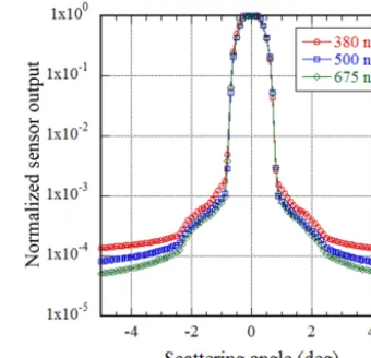
Figure 1.An example of measurement of the sun and the sky around the sun. The measurement was performed keeping the same azimuth angle as the solar azimuth angle. A positive (negative) value means a higher (lower) solar elevation, where the wavelengths are 380 nm (red), 500 nm (blue), and 675 nm (green). The values are normal-ized by the measured value at the zero scattering angle (direct solar irradiance).

source has a finite size: the SVA can be obtained by integrat-ing the output obtained while scannintegrat-ing the light source (see Appendix B).

To determine the SVA, a method using the measurement data around the sun was proposed by Nakajima et al. (1996). The radiances around the direction of the sun in 0.1×0.1◦ in-crements are measured; this is called a “solar disk scan”. Us-ing these data, the SVA is calculated. UsUs-ing similar gridded data, Torres et al. (2013) calculated the SVA of the Cimel-318 Sun-photometer and compared it with the values obtained by other methods.

An example of measurements of the radiance of the sun and around the sun is shown in Fig. 1. The measurements at POM-02 were performed vertically at intervals in the scat-tering angle of 0.1◦, where the wavelengths are 380, 500, and 675 nm. Here, “vertically” means that the measurements were performed while keeping the azimuth angle the same as the solar azimuth angle. In Fig. 1, the values are normalized by the measured value at the zero scattering angle (the direct solar irradiance), where a positive (negative) value means a higher (lower) solar elevation. At any wavelength, the output of POM-02 changes greatly around the scattering angles of

−2.5 and 2.5◦_{. This means that the output of POM-02 is}

af-fected by the direct solar irradiance up to about±2.5◦_from

the sun direction.

aerosols. However, Fig. 1 shows that the sensor output of POM-02 is affected by the direct solar irradiance for angles up to about±2.5◦_{from the sun’s center.}

The cause of the increase in the output between 0.75 and 2.5◦is considered to be stray light. As the length of the hood and the size of the lens are finite, even if the angle from the sun center exceeds 0.75◦, the direct solar light strikes the lens and results in “stray” light. This stray light reaches the detec-tor and increases the output, and is smaller than the measure-ment of the direct sun by three orders of magnitude or more, but the integrated value has a magnitude that can affect the estimation of the SVA. Furthermore, when solar light is used as the light source, aerosols and air molecules exist between the light source and the instrument. Therefore, the scattered light from aerosols and air molecules is included in the mea-surement of the direct solar irradiance. The influence of this scattered light must also be considered.

As seen from Fig. 1, roughly speaking, the FOV of POM-02 consists of a core from 0 to 0.5◦and a wing from 0.5 to 2.5◦.

1=1(core)+1(wing) (4)

=

Z

1(core)

f ()d+

Z

1(wing)

f ()d

Estimating the magnitudes of the two terms gives the follow-ing:

1(core)=

Z

1(core)

f ()d (5)

∼ =

Z

1(core) 1·d

=2π(1−cos(0.5◦))

=2.39×10−4,

1(wing)=

Z

1(wing)

f ()d (6)

∼ =

Z

1(wing)

fwingd

=2π(cos(0.5◦)−cos(2.5◦))fwing =5.74×10−3fwing.

As seen from Fig. 1,fwing≈10−3. Therefore, the ratio of the terms is as follows:

1(wing) 1(core) ≈

5.74×10−3fwing 2.39×10−4

=2.4×10−2. (7)

This means that neglecting the wing results in underestima-tion of the magnitude of the SVA by about 2 %. Iffwing≈

10−2, then the contribution of the wing to the SVA is about 20 %, and the instrument should be repaired. Iffwing≈10−4, then the contribution is about 0.2 %, and the wing can be ig-nored. The magnitude of the sensor output between 0.75 and 2.5◦ depends on the internal structure of the skyradiometer and the optical constant of the material.

When the direction of the sun is measured, the sensor out-putV (=0)is as follows:

V (=0) (8)

=C



 Z

1

f (0)I0g(0)d0+ Z

1

Isca(0)f (0)d0 



=v(0)+C1Isca(0),

where v(0)=C

Z

1

f (0)I0g(0)d0, (9)

Isca(0)= 1 1

Z

1

Isca(0)f (0)d0, (10)

andI0g(0)is the solar radiance distribution. The first term on the right-hand side of Eq. (8) is the contribution of the di-rect solar irradiance, and the second term is that of the scat-tered radiance.

When the direction of the sun is=0, the sensor output V (=0)is as follows:

V (=0) (11)

=C

  Z

1

f (0+0)I0g(0)d0+

Z

1

Isca(0+0)f (0)d0

 

=v(0)+C1Isca(0),

where the first term on the right-hand side is the contribution of the direct solar irradiance, and the second term is the scat-tered radiance. If0is outside of the field of view, then the first term is zero and only the second term is needed.

Currently, based on the data of the solar disk scan mea-surement, the SVA is calculated by the following equation:

10=

Z

1

v()+1CIsca() v(0)+1CIsca(0)

d. (12)

If there is no scattered radiance, then

10=

Z

1

v()

v(0)d, (13)

where10is the SVA1(see Appendices A, B).

scattering is dominant, the contribution of the scattered radi-ances increases.

We estimate the magnitude of each term of the integrand:

v()+1CIsca() v(0)+1CIsca(0)

= v()+1CIsca()

v(0)(1+1CIsca(0)/v(0)) .

(14) Usually, the solar disk scan measurement is performed only when the scattered light is much less than the direct solar irradiance:

1CIsca(0)/v(0)1.

The magnitude of this term has already been estimated from the influence of the scattered radiance in the field of view in the measurement of the sun-photometer; the estimation error of the optical depth due to the scattered radiance in the field of view (Zhao et al., 2012; Sinyuk et al., 2012).

Equation (14) can be approximated as follows: v()+1CIsca()

v(0)+1CIsca(0)

(15)

∼

=v()

+1CIsca()

v(0) 1−

1CIsca(0) v(0)

!

=v()+1CIsca()

v(0) (1−ε3)

=v()

v(0) +

1CIsca() v(0) −

v() v(0)ε3−

1CIsca() v(0) ε3,

where

ε3=

1CIsca(0)

v(0) . (16)

Therefore, Eq. (12) is as follows:

10 (17)

=

Z

1

v()+1CIsca() v(0)+1CIsca(0)

d

∼

=1+1

Z

1

CIsca()

v(0) d−1ε3

−1

Z

1

CIsca() v(0) dε3

=1    1+ Z 1

CIsca()

v(0) d−ε3−ε3 Z

1

CIsca() v(0) d

 

 .

As v(0)=CF0, whereF0 is the solar irradiance and C is the proportional constant (sensitivity) (see Appendix B), the

above Eq. (17) becomes

10∼=1    1+ Z 1

Isca() F0

d−ε3−ε3 Z

1

Isca() F0 d    (18)

=1{1+ε2−ε3−ε2ε3}, in which

ε2= Z

1

Isca() F0

d. (19)

The fourth term is smaller than the second and third terms and it can be ignored. Then, comparing the second and third terms in the curly brackets,

ε2= Z

1

Isca() F0 d (20) = Z 1    1 F0 · 1 1 Z 1

Isca(+0)f (0)d0  

 d,

ε3= 1 F0 · 1 1 Z 1

Isca(0+0)f (0)d0 (21)

=1Isca(=0)

F0 ,

whereε2is the integral of the mean scattered lightIsca() in the region off () >0, andε3is the integral of scattered light in the FOV when facing toward the sun.

Thef () of the POM-02 consists of the core from 0.0 to 0.5◦_{, which takes large values, and the wing from 0.5 to}

2.5◦_{which takes small values. Therefore, the integral can be}

written as follows:

ε2= Z

1

Isca() F0

d (22)

=

Z

1(core) Isca()

F0 d+

Z

1(wing) Isca()

F0 d,

AsIsca()≈Isca(=0)in the core, R 1(wing)

f ()d1,

and R

1(core)

d∼=1, the first term of the integral ε2 is as follows:

Z

1(core) Isca()

F0

d∼=Isca(=0)

F0

1. (23)

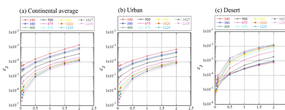
Figure 2.Estimation of the errorε2in the calculation of the SVA. Aerosol models are the OPAC continental average, urban, and desert. The aerosol optical depth thickness is that at a wavelength of 550 nm and the solar zenith angle is 30◦.

Figure 3.Same as Fig. 2 but for errorε3.

whereas the integral of the wing remains. The area of the integral of the wing is larger than that of the core. Even if the integral of scattered light in the FOV is small compared to the solar direct irradiance, the integral of the wing becomes large and introduces errors in the SVA estimation. That is, even if the measurement value of scattered light is smaller than the direct sun measurement,Isca()1/F0≈10−3, the integral of the wing becomes large:

Z

1(wing) Isca()

F0

d≈1(wing)

1 ×10

−3 ₍₂₄₎

≈1(wing)

1(core) ×10

−3_=2.4×10−2_.

In this case, the magnitude of the error is about 2 %.

Figures 2 and 3 show the values ofε2 andε3 when the aerosol optical depth at 550 nm is changed. Here, the solar zenith angle is 30◦and the aerosol models are the OPAC con-tinental average, urban, and desert types (Hess et al., 1998). The simulation calculations of the scattered sky radiances were performed using the subroutine in the SKYRAD pack-age. The Ångström exponents of the continental average in the shorter (350 to 500 nm) and longer (500 to 800 nm) wave-length regions are 1.11 and 1.42, respectively. Those of the urban areas are 1.14 and 1.43, respectively, and those of the desert are 0.20 and 0.17, respectively.

path length=optical depth×airmass) at 550 nm is less than 0.5(0.50/cos(30◦_{)=0.58), then the second termε}

2is less than 0.5 %, and if the aerosol optical depth at 550 nm is less than 1, then the second termε2is less than 1 %. In the desert model, which includes large particles, the second term is less than 1 % for shorter wavelengths, where desert particles have a higher absorption than in the longer wavelength regions. However, even if the aerosol optical depth at 550 nm is less than 0.5, the second term is larger than 1 % for some wave-lengths.

From these simulations if the scattered light can be re-moved from the SVA calculation, then an improvement in the accuracy of the calculations can be expected. However, as the intensity of the scattered light depends on aerosol character-istics, it is difficult to estimate the intensity of the scattered light from the measurements. Furthermore, close to the sun the value of scattered light cannot be measured due to the direct sunlight. In POM-01 and POM-02, scattered light can only be measured without being affected by direct sunlight at scattering angles of more than 3◦.

The SVA was calculated by subtracting the measurements for a scattering angle of 3◦and the accuracy of the estimation was examined. Although not shown in detail, for the conti-nental average and urban models, even if the aerosol optical depth (optical path length) is 2 (2.3) at 550 nm, the error in the SVA estimation was less than 0.5 %. This indicates that if the measured value of scattered light can be subtracted, the estimation accuracy of the SVA can be greatly improved.

From these results, when we determine the SVA by using the data from the solar disk scan measurement if the aerosol optical depth (optical path length) is less than 0.5 (0.58) and the aerosol does not include large particles such as desert dust particles, the effect of the scattered radiances on the SVA calculation is less than 0.5 %, and1is well approximated by10. Furthermore if the measured value of the scattered light can be subtracted, the estimation accuracy of SVA can be greatly improved.

3 SVA calculation with the SKYRAD package

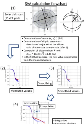
The software in the SKYRAD package (Nakajima et al., 1996) is often used for SVA calculation from the data of the solar disk scan measurement. However, the authors no-ticed that there are problems in this program, and this sec-tion investigates these problems in detail. In Appendix C, a flowchart is shown illustrating the SVA calculation procedure in the SKYRAD package.

In the measurement of the solar disk scan, a range of±1◦ in the zenith angle direction and ±1◦in the azimuth direc-tion relative to the sun in increments of 0.1◦is used, which produces a 21×21 grid with an angular resolution of 0.1◦. Therefore, the data are taken from the sun for scattering an-gles of up to about 1.4(=(1◦)×

√

2)◦. As shown in Fig. 1, the influence of the direct solar irradiance as a light source

extends to about 2.5◦. To take this into consideration, the in-tegration is performed by extrapolation for angles larger than 1.4◦_.

The following three problems exist in the SKYRAD pack-age for calculating the SVA.

First, the data processing does not consider changes in the airmass (solar zenith angle) during the solar disk scan surement. However, in practice, if the solar disk scan mea-surement is conducted when the airmass change (solar zenith angle) is small, then the resulting error is also small. Also, this is not usually a problem unless the measurement is con-ducted over an extended period of time.

Second, before starting the data processing, the minimum measured value is subtracted from the measured values. As a result, the measurements of the scattering angle between 1 and 1.4◦ are greatly affected. By integrating the measured value minus the minimum, the SVA is always underesti-mated, but the solution to this problem is not straightforward. Thirdly, the values between 1.4 and 2.5◦are not properly extrapolated. Frequently, the extrapolated value does not de-crease monotonically. In some cases, this partially cancels out the underestimation of the integral.

In Fig. 4, an example of the integrand for the SVA cal-culation is shown. In the blue curve with open squares, the minimum value is subtracted. This curve is then integrated by the current SKYRAD program. As the minimum value is subtracted, the difference is noticeable at scattering angles greater than 1◦. In this case, the extrapolated value from 1.4 to 2.5◦ is almost constant. In many cases, nearly constant values were extrapolated as in this example. In some cases, the extrapolated values increased. In the red curve with open circles, the minimum value is not subtracted. The values be-tween 1.4 and 2.5◦ _{were extrapolated using the data from}

1.0 to 1.4◦. Considering Fig. 1, the decreasing trend is more realistic. Furthermore, Manago et al. (2016) showed, using lamp-based measurements at the ground level, that the FOV monotonically decreases to around 2.5◦and then sharply de-creases as the scattering angle inde-creases.

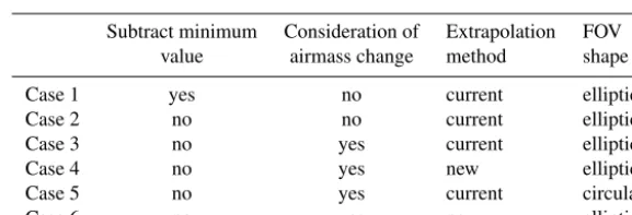
To investigate the differences in the calculation methods, several calculations were performed.

The following steps in the calculations were varied: 1. whether the minimum value was subtracted; 2. whether the change in airmass was considered;

3. the method for the extrapolation in the range from 1.4 to 2.5◦;

4. whether the horizontal cross-section of the FOV is as-sumed to be a circle or an ellipse (the current SKYRAD package method uses an ellipse);

Figure 4.Example of the integrand of the SVA calculation. The blue line with open squares is for the case that the minimum value is subtracted, and the red line is for the case that the values between 1.4 and 2.5◦are extrapolated using the data from 1.0 to 1.4◦.

Table 1.Settings of the SVA calculation.

Subtract minimum Consideration of Extrapolation FOV

value airmass change method shape

Case 1 yes no current elliptic

Case 2 no no current elliptic

Case 3 no yes current elliptic

Case 4 no yes new elliptic

Case 5 no yes current circular

Case 6 no yes new elliptic

Case 1 is the method implemented in the current SKYRAD package. In Case 5, “circular” means that the FOV is axisymmetric. The elliptic shape parameters in Case 6 are calculated by a different method from the SKYRAD package.

The solar disk scan measurement was made between 10:00 and 13:00 local time (LT) at MLO. The optical depth at wave-lengths of 500 and 340 nm were at most 0.1 and 0.5, respec-tively. Therefore, the influence of the scattered light on the SVA calculation is small.

The SAV was calculated for the six cases shown in Ta-ble 1, including Case 1, which is the current method used by the SKYRAD package. In Cases 4 and 6, the values in the range 1.4 to 2.5◦were extrapolated as a linear function of the cosine of the scattering angle. This linear function was de-termined by the least squares method using the data with a scattering angle of more than 1◦. In Cases 3, 4, 5, and 6, as-suming that the aerosol optical depth has not changed, the so-lar direct irradiance changes due to the change of the airmass during the measurement. The elliptic parameters in Case 6 were determined by assuming that the shape of the FOV is a 2-dimensional Gaussian distribution. The results of the com-parison are summarized in Table 2.

The difference between Case 1 and Case 2 is whether or not the minimum value was subtracted. Case 1, in which the minimum value was subtracted, results in an underestimation of about 1 % to 4 %.

The standard deviation in the region of shorter wave-lengths in Case 1 is smaller than for the other cases. One of the causes of the variation of the calculated SVA is the variation of the wing of the FOV. In the region of shorter wavelengths, generally, the optical depth is thicker than the longer wavelength region, and the scattered light increases in the shorter wavelength region. When the minimum value is subtracted from the measurement value, the value of the wing portion decreases greatly in the shorter wavelength region, and the contribution to the SVA integration also decreases greatly in the short wavelength region. As a result, the vari-ance of the calculated SVA becomes small. However, there is no justification for subtracting the minimum value.

The difference between Case 2 and Case 3 is whether the change in airmass was considered or not. The solar disk scan measurement was made between 10:00 and 13:00 LT at MLO. Therefore, the change in the air mass is less than 0.01, and there was hardly any influence from the change in air-mass.

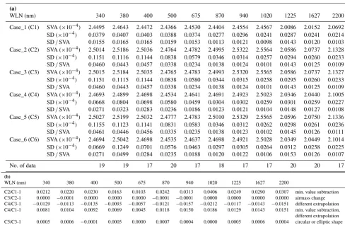
Table 2.Influence of the different calculation settings.(a)Calculated SVA. The data taken at MLO in October and November 2015 are used. (b)Comparison of calculated SVA.

(a)

WLN (nm) 340 380 400 500 675 870 940 1020 1225 1627 2200

Case_1 (C1) SVA(×10−4) 2.4495 2.4643 2.4472 2.4366 2.4530 2.4404 2.4554 2.4567 2.0086 2.0152 2.0692 SD (×10−4) 0.0379 0.0407 0.0403 0.0388 0.0374 0.0277 0.0296 0.0241 0.0287 0.0241 0.0214 SD/SVA 0.0155 0.0165 0.0165 0.0159 0.0153 0.0113 0.0121 0.0098 0.0143 0.0120 0.0103 Case_2 (C2) SVA (×10−4) 2.5014 2.5186 2.5036 2.4764 2.4782 2.4995 2.5322 2.5564 2.0586 2.0737 2.1328 SD (×10−4) 0.1151 0.1116 0.1144 0.0838 0.0579 0.0346 0.0314 0.0257 0.0294 0.0260 0.0233 SD/SVA 0.0460 0.0443 0.0457 0.0338 0.0234 0.0138 0.0124 0.0101 0.0143 0.0125 0.0109 Case_3 (C3) SVA (×10−4) 2.5015 2.5184 2.5035 2.4765 2.4783 2.4993 2.5320 2.5565 2.0586 2.0737 2.1327 SD (×10−4) 0.1151 0.1115 0.1144 0.0838 0.0580 0.0344 0.0315 0.0258 0.0295 0.0260 0.0233 SD/SVA 0.0460 0.0443 0.0457 0.0338 0.0234 0.0138 0.0124 0.0101 0.0143 0.0125 0.0109 Case_4 (C4) SVA (×10−4) 2.4693 2.4899 2.4698 2.4534 2.4641 2.4691 2.4923 2.5023 2.0346 2.0440 2.1005 SD (×10−4) 0.0668 0.0804 0.0698 0.0580 0.0459 0.0304 0.0302 0.0259 0.0301 0.0259 0.0227 SD/SVA 0.0271 0.0323 0.0283 0.0236 0.0186 0.0123 0.0121 0.0104 0.0148 0.0127 0.0108 Case_5 (C5) SVA (×10−4) 2.5027 2.5199 2.5032 2.4777 2.4783 2.5010 2.5329 2.5565 2.0596 2.0750 2.1336 SD (×10−4) 0.1155 0.1123 0.1141 0.0831 0.0583 0.0346 0.0312 0.0262 0.0298 0.0261 0.0236 SD/SVA 0.0461 0.0446 0.0456 0.0335 0.0235 0.0138 0.0123 0.0102 0.0145 0.0126 0.0111 Case_6 (C6) SVA (×10−4) 2.4694 2.5042 2.4698 2.4535 2.4637 2.4698 2.4921 2.5028 2.0349 2.0449 2.1014 SD (×10−4) 0.0669 0.1249 0.0701 0.0576 0.0463 0.0297 0.0305 0.0264 0.0312 0.0258 0.0225 SD/SVA 0.0271 0.0499 0.0284 0.0235 0.0188 0.0120 0.0122 0.0106 0.0153 0.0126 0.0107

No. of data 19 19 17 20 17 18 17 17 20 20 17

(b)

WLN (nm) 340 380 400 500 675 870 940 1020 1225 1627 2200

C2/C1-1 0.0212 0.0220 0.0230 0.0163 0.0103 0.0242 0.0313 0.0406 0.0249 0.0290 0.0307 min. value subtraction C3/C2-1 0.0000 −0.0001 0.0000 0.0000 0.0000 −0.0001 −0.0001 0.0000 0.0000 0.0000 0.0000 airmass change C4/C3-1 −0.0129 −0.0113 −0.0135 −0.0093 −0.0057 −0.0121 −0.0157 −0.0212 −0.0117 −0.0143 −0.0151 different extrapolation C4/C1-1 0.0081 0.0104 0.0092 0.0069 0.0045 0.0118 0.0150 0.0186 0.0129 0.0143 0.0151 min. value subtraction, different extrapolation C5/C3-1 0.0005 0.0006 −0.0001 0.0005 0.0000 0.0007 0.0004 0.0000 0.0005 0.0006 0.0004 circular or elliptic shape C6/C4-1 0.0000 0.0057 0.0000 0.0000 −0.0002 0.0003 −0.0001 0.0002 0.0001 0.0004 0.0004 different elliptic parameters

current SKYRAD package, the SVA was overestimated by 0.6 % to 2.1 %.

As there was hardly any influence from the change in air-mass, in Case 1 and Case 4 the underestimation caused by the subtraction of the minimum value and the overestimation caused by the poor extrapolation partially cancel each other out, and the current SKYRAD package method underesti-mates the SVA by 0.5 % to 1.9 %.

The difference between Case 3 and Case 5 is whether the horizontal cross-section of the FOV is assumed to be a cir-cle or an ellipse. The difference between them was less than 0.1 %. This indicates that POM-02 was well tuned when it was shipped from the manufacturer.

In Case 6, a different method for determining elliptic parameters from the current SKYRAD package was used. Therefore, the difference between Case 4 and Case 6 is the difference between the methods used to determine the ellip-tic parameters. There was almost no difference between the current method and the new method. The method used to de-termine the elliptic parameters thus has little effect on the SVA estimation.

4 Annual trend and seasonal variation of SVA

Broadly speaking, the SVA is determined by the size of the pinhole and the focal length of the lens. There is a possibility that these parameters may change with degradation and the inside temperature. Therefore, the annual trend and seasonal variation of the SVA are examined.

Figures 5 and 6 show the SVAs in the visible and near-infrared region (Si photodiode) and in the shortwave-near-infrared region (InGaAs photodiode) for 2008 and 2016, respectively. The observation for the calibration at MLO was performed over about a month in October and November each year. The lens in the visible region was replaced before the observation in 2013.

Ad-Figure 5.SVAs in the visible and near-infrared region (Si photodiode) from 2008 to 2016. The data were taken at MLO over a month in October and November every year.(a)SVA calculated by the corrected method in this study,(b)SVA at a wavelength of 500 nm calculated by both the corrected and the current SKYRAD package methods.

Figure 6.Same as Fig. 5 but for the shortwave-infrared region (InGaAs photodiode). The wavelength in(b)is 1627 nm.

ditionally, from this figure, the uncertainty of the SVA (the ratio of standard deviation/mean) is estimated at about 1 % except in 2015.

From 2008 to 2012, the value of the SVA seems to be de-creasing. The value of the SVA in 2008 is larger than in other years. The mean values of the SVA are within±0.5 % except in 2008. From 2013 to 2016, the mean values of the SVA are within±1 %. The annual variation of the SVA is less than or equal to the uncertainty of the SVA. From these results, the annual trend in the SVA cannot be seen in only 4 years of data, and even if there is a trend, it is smaller than the mea-surement uncertainty.

Figure 6a is the same as Fig. 5a except for channels 9 to 11 (1225, 1627, 2200 nm) and Fig. 6b is the same as Fig. 5b except for channel 10 (1627 nm). In these channels, the SVA

calculated by the current method is also lower than that cal-culated by the corrected one except in 2008.

The determination uncertainty of the SVA is also estimated as about 1 %. The lens in the shortwave-infrared region was not replaced in the period from 2008 to 2016. The trend in the SVA cannot be seen in 8 years of data either. The values of the SVA in this period are within±1 %, which is the de-termination uncertainty of the SVA. From these results, the annual trend of the SVA in the shortwave-infrared channels cannot be seen in 8 years of data, and even if there is a trend, it is smaller than the measurement uncertainty.

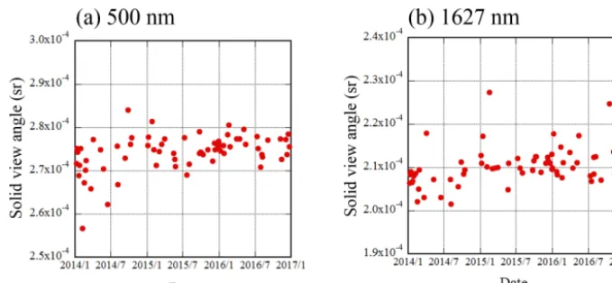
Figure 7.Time series of the SVA at POM-02 (Tsukuba) from January 2014 to December 2016.(a)500 nm, the mean and standard deviation are 2.743×10−4and 4.2×10−6, respectively.(b)1627 nm, the mean and standard deviation are 2.104×10−4and 4.4×10−6, respectively.

a large amount of data in the winter, because there are many fine days in the winter in Tsukuba. There are little data from spring to autumn and the data in the summer are scattered. As the estimated SVA is scattered, it is not possible to draw a clear conclusion, but as can be seen from Fig. 7, the sea-sonal variation exceeding±2 % cannot be confirmed in ei-ther channel. This also indicates that the temperature depen-dence of the SVA in both detector regions cannot be seen. As the data are taken over a short period of 3 years, no annual trend in the SVA can be detected.

5 Summary and conclusion

Atmospheric aerosols are an important constituent of the atmosphere. Measurement networks covering an extensive area from ground and space have been developed. SKYNET is a ground-based monitoring system using sky radiometers POM-01 and POM-02 (Prede Co. Ltd., Japan). To improve the measurement accuracy, it is important to know the char-acteristics of the instruments and calibrate them. There are two constants that we must determine to make accurate mea-surements. One is the calibration constant, and the other is the SVA of the radiometer.

In Part 1, problems related to the estimation of the cali-bration constant were investigated, and in Part 2, problems related to the determination of the SVA of the sky radiometer were described.

In this study, the data from two sky radiometers POM-02 of the JMA/MRI were analyzed. One of the sky radiometers was used as a calibration reference, and the other was used for the continuous measurement at the Tsukuba MRI obser-vation site.

The FOV of POM-02 consists of a core from 0 to 0.5◦ and a wing from 0.5 to 2.5◦. The wing is about 3 orders of magnitude smaller than the core, but the wing contributes about 2 % to the SVA.

A method for determining the SVA using the sun as a light source was proposed by Nakajima et al. (1996). In this method, the radiance around the direction of the sun in 0.1×0.1◦increments is measured. These measurements in-clude the scattered light from aerosols and air molecules as well as the direct solar irradiance. These scattered radiances cause errors in the SVA calculation.

The influence of the scattered light was evaluated by sim-ulations. As a result if the aerosol optical depth (optical path length) is less than 0.5 (0.58) at a wavelength of 550 nm and the aerosol does not include large particles such as desert dust particles, then the effect of the scattered radiances on the SVA calculation is less than 0.5 %. Furthermore if the mea-surements of the scattered light can be taken into account, the estimation accuracy of the SVA can be greatly improved.

The SKYRAD package for determining the SVA from the solar disk scan measurements has several problems. The problems do not result in major errors in the estimation of the SVA, but can cause a systematic underestimation.

First, the data processing does not consider the change in the airmass (solar zenith angle) during the solar disk scan measurement. In practice if the measurements are taken over a period when the change in airmass is small, then there is al-most no problem. Second, before beginning the data process-ing, the minimum value is subtracted from each measured value. This results in an underestimation of the SVA by 1 % to 4 %. Thirdly, the values between 1.4 and 2.5◦are not prop-erly extrapolated. This overestimates the SVA value by 0.6 % to 2.1 %. As the second and third errors partially cancel each other out if the current software is used, the overall error will be an underestimation of 0.5 % to 1.9 %.

from 2009 to 2012 and 2013 to 2016, and it was smaller than the measurement accuracy. In the shortwave-infrared region, the annual trend of the SVA could not be seen in 8 years data from 2008 to 2016, and it was smaller than the measurement uncertainty.

The seasonal variation of the SVA was examined using the data taken at Tsukuba from January 2014 to December 2016. As the time series of the determined SVA was scattered over a range of ±2 %, it is not possible to draw a clear conclu-sion, but seasonal variation exceeding ±2 % could not be confirmed. Furthermore, as the temporal range of the data was short, no annual trend could be detected.

According to the method based on the current measure-ment data, the uncertainty is 1 % at high-altitude mountain sites such as MLO and 1.5 % to 2 % at low-altitude sites such as Tsukuba. The cause of the error may be an increase in the scattered light in the optically thick case, a variation in the solar direct irradiance due to a change in the aerosol con-centration during the solar disk scan measurement, and an error in the pointing direction of the FOV. In the future, we will eliminate scattered light and use measurements of the aerosol optical depth from other instruments during the solar disk scan measurement. We will also develop methods for measuring the SVA on the ground or in a laboratory.

Appendix A

Letf ()be the response function of the FOV, where in-dicates the direction, and when=0,f (=0)=1.

The SVA is then as follows: 1=

Z

1

f ()d. (A1)

Suppose parallel light enters from=0. V (=0)

=C

Z

1

f ()δ(−0)F0d (A2)

=Cf (=0)F0

Here,F0is the input irradiance, andC is the proportional constant (sensitivity).

Therefore, f (0)=

V (0) CF0

. (A3)

Asf (0)=1, thenV (0)=CF0. Therefore, 1= Z 1 f ()d = Z 1

V (0) CF0

d0 (A4)

=

Z

1

V (0) V (0) d0.

When the parallel light is incident, the SVA of the ra-diometer can be obtained by integrating the output in an ar-bitrary direction normalized by the output in the direction of =0.

Appendix B

Here, we consider the case that the light source has a finite size, for example, when the sun is used as a light source.

Let the radiance distribution of the light source beI ()=

I0g().

The integrated energy of the light sourceF0is as follows:

F0= Z

1

g()I0d, (B1)

where1is the extent of the light source.

Considering the sun as a light source, let1be smaller than 1. Also, when the sun is a light source, F0 is the solar irradiance.

LetC be the sensitivity of the detector, where C is the proportional constant of the sensor output and input energy.

The light source is in the direction of=0 and we mea-sure the radiance from it as

v(0)=C Z

1

f (0+0)g(0)I0d0, (B2)

wherev(0)is the sensor output.

Iff ()is constant within the range of1(POM-02 sat-isfies this condition), then this equation can be rewritten as follows:

v(0)=CI0 Z

1

f (0)g(0)d0 (B3)

=CI0f (0) Z

1

g(0)d0

=Cf (0)F0 =CF0.

Next, the light source is in the direction of=0: v(0)=CI0

Z

1

f (0+0)g(0)d0, (B4)

wherev(0)is the sensor output.

Then, both sides of the equation are integrated within the SVA1:

Z

1

v(0)d0 (B5)

= Z 1  CI0 Z 1

f (0+0)g(0)d0 

d0.

By changing the order of integration on the right, the fol-lowing equation can be obtained:

Z

1

v(0)d0=CI0 Z

1



g(0) Z

1

f (0+0)d0 

d

0

=CI0 Z

1

g(0)d0·1 (B6)

=CF01.

Therefore, from Eqs. (B3) and (B6), 1= 1

CF0 Z

1

v(0)d0, (B7)

=

Z

1

v(0) v(0) d0.

Appendix C

Author contributions. This study was designed by AU and TM. The measurements of sky radiometer were conducted by AU and AK. Simulations and the analyses were performed by AU. The manuscript was written by AU, and all authors contributed to edit-ing and revision.

Competing interests. The authors declare that they have no conflict of interest.

Special issue statement. This article is part of the special issue “SKYNET – the international network for aerosol, clouds, and so-lar radiation studies and their applications (AMT/ACP inter-journal SI)”. It is not associated with a conference.

Acknowledgements. This work was supported by the NIES

GOSAT-2 project, Japan. This work was also partially supported by JSPS KAKENHI grant number JP17K00531.

Edited by: Omar Torres

Reviewed by: one anonymous referee

References

Hashimoto, M., Nakajima, T., Dubovik, O., Campanelli, M., Che, H., Khatri, P., Takamura, T., and Pandithurai, G.: Develop-ment of a new data-processing method for SKYNET sky ra-diometer observations, Atmos. Meas. Tech., 5, 2723–2737, https://doi.org/10.5194/amt-5-2723-2012, 2012.

Hess, M., Koepke, P., and Schult, I.: Optical Properties of Aerosols and Clouds: The Software Package OPAC, B. Am. Meteorol. Soc., 79, 831–844, 1998.

Holben, B. N., Eck, T. F., Slutsker, I., Tanré, D., Buis, J. P., Setzer, A., Vermote, E., Reagan, J. A., Kaufman, Y. J., Nakajima, T., Lavenu, F., Jankowiak, I., and Smirnov, A.: AERONET-A feder-ated instrument network and data archive for aerosol characteri-zation, Remote Sens. Environ., 66, 1–16, 1998.

Khatri, P., Takamura, T., Nakajima, T., Estellés, V., Irie, H., Kuze, H., Campanelli, M., Sinyuk, A., Lee, S.-M., Sohn, B. J., Pan-dithurai, G., Kim, S.-W., Yoon, S. C., Martinez-Lozano, J. A., Hashimoto, M., Devara, P. C. S., and Manago, N.: Factors for inconsistent aerosol single scattering albedo between SKYNET and AERONET, J. Geophys. Res.-Atmos., 121, 1859–1877, https://doi.org/10.1002/2015JD023976, 2016.

Lohmann, U. and Feichter, J.: Global indirect aerosol ef-fects: a review, Atmos. Chem. Phys., 5, 715–737, https://doi.org/10.5194/acp-5-715-2005, 2005.

Manago, N., Pradeep, K., Irie, H., Takamura, T., and Kuze, H.: On the method of solid view angle calibration for SKYNET skyra-diometers, 4th International SKYNET workshop, Rome, Italy, 2–4 March, 2016.

Nakajima, T., Tonna, G., Rao, R., Kaufman, Y., and Holben, B.: Use of sky brightness measurements from ground for remote sensing of particulate polydispersions, Appl. Opt., 35, 2672–2686, 1996. Ramanathan, V., Crutzen, P. J., Kiehl, J. T., and Rosenfeld, D.: Aerosols, Climate, and the Hydrological Cycle, Science, 294, 2119–2124, 2001.

Sinyuk, A., Holben, B. N., Smirnov, A., Eck, T. F., Slutsker, I., Schafer, J. S., Giles, D. M., and Sorokin, M.: Assessment of error in aerosol optical depth measured by AERONET due to aerosol forward scattering, Geophys. Res. Lett., 39, L23806, https://doi.org/10.1029/2012GL053894, 2012.

Takamura, T., Nakajima, T., and SKYNET community group: Overview of SKYNET and its Activities. Proceedings of AERONET workshop, El Arenosillo, Opt. Pura Aplicada, 37, 3303–3308, 2004.

Torres, B., Toledano, C., Berjón, A., Fuertes, D., Molina, V., Gon-zalez, R., Canini, M., Cachorro, V. E., Goloub, P., Podvin, T., Blarel, L., Dubovik, O., Bennouna, Y., and de Frutos, A. M.: Measurements on pointing error and field of view of Cimel-318 Sun photometers in the scope of AERONET, Atmos. Meas. Tech., 6, 2207–2220, https://doi.org/10.5194/amt-6-2207-2013, 2013.

Uchiyama, A., Matsunaga, T., and Yamazaki, A.: The in-strument constant of sky radiometers (POM-02) – Part 1: Calibration constant, Atmos. Meas. Tech., 11, 5363–5388, https://doi.org/10.5194/amt-11-5363-2018, 2018.