Indexing moving objects: A real time approach
1George Lagogiannis1, Nikos Lorentzos1, and Alexander B. Sideridis1
1Agricultural University of Athens, Iera Odos 75, 11855 Athens, Greece
{lagogian, lorentzos, as}@aua.gr
Abstract. Indexing moving objects usually involves a great amount of updates, caused by objects reporting their current position. In order to keep the present and past positions of the objects in secondary memory, each update introduces an I/O and this process is sometimes creating a bottleneck. In this paper we deal with the problem of minimizing the number of I/Os in such a way that queries concerning the present and past positions of the objects can be answered efficiently. In particular we propose two new approaches that achieve an asymptotically optimal number of I/Os for performing the necessary updates. The approaches are based on the assumption that the primary memory suffices for storing the current positions of the objects.
Keywords: Persistence, I/O complexity, Indexing structures.
1. Introduction
Objects that change their position and/or shapes over time introduce large spatio-temporal data sets. The efficient manipulation of such data sets is crucial for an increasing number of computer applications (location aware services, traffic monitoring etc). Considering in particular, moving objects as vehicles that move in a city, we can think of many interesting queries such as “find the closest police car”, or “find the number of vehicles that went through the center of the city between 11:00 and 13:00”.
In the real time version of our spatiotemporal problem, we can consider a client-server architecture where each moving client (object) sends its position to the server, at discrete times. The server collects information reports (messages) of the form (object Id, current-cell, current time) from the moving
objects, every P seconds. We assume that the objects move in a 2 d space.
Queries on such data sets may be of a “historical” kind or may be posed strictly on the current position of the objects. This paper does not deal with the
present time. By current position of an object we mean the position indicated
by the last message sent by the object. The actual current position is unknown, and one can only guess, according to the latest position, and the speed vector of the object. Thus we only deal with the past. The term “real
time”, is used to denote that the updates on the data structures (in secondary memory) caused by the messages (sent by the vehicles) are not postponed, but instead, these structures are updated with every incoming message.
In building a system to index moving objects, we have two alternatives for indexing the space involved (a 2-d space in our case), static and dynamic
indexing. In static indexing, the 2-d space is divided into “cells” and the area
occupied by each such cell does not change during the monitoring period, i.e., it is static. In dynamic indexing, the 2-d space is divided into regions in such a way that, at all times, there is a minimum number of objects in every region. To satisfy this property, we need to update the regions as objects move (hence the regions are dynamic). In this paper we provide solutions based on both static and dynamic indexing strategies, aiming at minimizing the number of I/Os needed to store the messages sent by the objects. Assuming that with each I/O we can store B such messages (i.e. B messages fit into a disk block), we conclude that the minimum number of I/Os can be achieved if we
manage to store B messages with each I/O. If we manage to store c*B
messages per I/O, (where c is a constant less than 1) then we say that our solution is asymptotically optimal. Such solutions are present in this paper.
Optimizing the I/Os of existing multidimensional indexing structures (mainly the R-tree) is the target of many recent efforts (see [3], [4], [6], [11], [12], [14]). A common part of most of these solutions is a secondary index structure, used for accessing the leaf of the main indexing structure that contains a given object. This secondary index structure is used to avoid the multiple paths search operation in the R-tree during the top-down update. This way a bottom-up approach is proposed.
Compared with the related work described above, our work differs because of the combination of the following three characteristics:
i) We use a worst case efficient data structure instead of an R-tree, since the R-tree is not very efficient under a large amount of updates. The worst case framework which we apply is important for real time applications, where the data structures involved should be completely predictable with respect to their time complexities. Searching for example for the closest taxi requires a predictable amount of time because the positions of the objects change rapidly and the taxi closest, one minute ago, may not currently be the closest taxi. Tight bounds tend to make such applications more reliable and, in this sense, reliability is really promoted by using a worst case efficient indexing structure and in particular, partially persistent B-trees (see [2], [13]).
ii) We aim at storing not only the present positions of the objects, but also the past ones. The past positions are crucial for the answering of historical queries and such queries are certainly of interest.
number of I/Os. We do not make any assumptions or real life observations relevant to the way of the movement of the objects. Thus, our work should be seen as an approach into which many observations from real applications can be incorporated, in order for practical implementations to be created.
2. Problem definition
As is obvious, storing the past positions of objects requires the use of secondary storage because of the huge amount of data involved. Given that a large number of objects is being tracked, the main concern is to face the bottlenecks caused by the large volume of I/Os for storing into secondary memory the messages sent by the objects. The parameters involved are summarized as follows.
N: The maximum number of tracked objects.
M: The amount of main memory used.
P: The time period of communication between the objects and the base
station, measured in seconds.
R: The number of I/Os per second supported by the hard disk of our
system.
B: The number of messages that fit into a disk block.
W: The total number of messages received by the system during the
tracking time.
An I/O may be of one of the following two types:
Message storing I/O, which stores some (optimally O(B)) messages, into a disk block.
Rebalancing I/O: This I/O is caused by the indexing structure.
The first type of I/O is caused by the incoming messages. For an example of an I/O of the second type, consider a message-storing I/O that inserts a new record into a leaf of a B-tree. This may cause a split of the leaf and of some of the ancestors of this leaf. The additional I/Os, required to rebalance the B-tree, are the rebalancing I/Os.
Since at most B messages can be stored into secondary memory by one
I/O, it follows that the minimum number of I/Os that can be achieved is W/B.
In fact, this number can be achieved by the following trivial solution: Each new message sent by an object is copied into a buffer, whose capacity is equal to
B messages. When this buffer is filled, we store its B messages at the end of
a secondary memory file and the buffer is then freed. Clearly, this solution
achieves W/B I/Os all of which are message-storing, since no indexing
structure is used.
show that this sacrifice is enough to achieve query efficient solutions. In conclusion, the solutions we present have the following property.
Property 1: To store the total number of messages (W) received by the system, the required number of message-storing I/Os is O(W/B).
For our purposes, it is assumed that the primary memory is sufficiently large to store the current position of tracked objects. Assume, for example, that 5 million moving vehicles are being tracked in a city. Assume also that,
for each vehicle, a tuple of c bytes is maintained in primary memory,
containing the Vehicle Id and the necessary additional data. Then the primary
storage required is not more than 5*c Mbytes. Assuming that we use
sophisticated data structures, this number has to be multiplied by only a small constant. Such an amount of primary memory is not considered to be prohibitive nowadays neither from a technical nor from an economical point of view.
As mentioned in the introduction, one can index the 2-d space where the objects move, statically and dynamically. In this paper we follow both approaches.
Our static indexing approach is based on a grid. We assign an indexing structure to each cell of the grid. Such an indexing strategy is suitable for the processing of range queries. In this paper we explore this strategy for the processing of spatiotemporal range predicates. A spatiotemporal range predicate is a pair (S, T) where S is a spatial constraint and T is a temporal constraint which can be either a time instance or a time interval. The output of the query is either the set of objects inside S at the time instance T, or the set of objects inside S at some time instance during the time interval T.
By indexing the space in a dynamic way, we are able to efficiently process
spatio-temporal nearest (k-nearest) neighbour predicates. Such a predicate is
a pair (Q, T), where Q is a point on the map and T can again be either a time instance or a time interval. The output is the nearest object (or the k-nearest objects) to Q, at the time instance T or during the time interval T.
The time complexities of the solutions provided are derived in the external-memory model of computation given in [1], i.e. we neglect the time spent for primary memory actions and the only measurement of efficiency we care about is the number of I/Os.
3. Partial Persistence
Traditional data structures are ephemeral, in the sense that we do not
maintain older versions, we only update the current version. Maintenance of the old versions leads to persistent data structures. There are three kinds of
persistence: In partial persistence, the latest version can be updated, and the
old versions can only be searched. In full persistence, all versions can be searched and be updated. Finally, in confluent persistence, one property is added, that two different versions can be merged.
In the seminal paper by Driscoll, Sarnak, Sleator and Tarjan, [5], two general methods are presented, that transform an ephemeral data structure
into a partially persistent: The fat-node method (also achieving full
persistence) and the node-copying method. By applying the fat-node or the node-copying method to an ephemeral (initial) structure we can create its partially persistent version.
A fat node corresponds to a node of the (initial) ephemeral structure. It can become arbitrarily big, and it contains the entire history of the corresponding ephemeral node. The node-copying method produces fixed-size nodes and it is optimal, i.e., the time complexity of the produced partially persistent structure is asymptotically equal to the time complexity of the (initial) ephemeral structure.
Applying the methods of [5] in secondary memory turned out to be a separate research area, because its straightforward application leads to a huge amount of wasted space. Having been inspired by the fat-node method, Lanka and Mays [10], proposed a method, called fat field, that reduces the space requirements of their data structure. In this method, the empty fields of a block in a fat node are used to store modifications of data fields, as long as they do not cause overflows. Using this method, they presented fully persistent B-trees which can also be used for the partially persistent case except that the time complexities achieved this way, are not optimal.
To achieve optimal partially persistent B+-trees, one must adjust the node-copying method to secondary memory. Such partially persistent B-trees have also been developed, in particular the Multi Version B-Tree (MVBT) by Becker et al. [2] and the Multi Version Access Structure (MVAS) by Varman and Verma [13]. These methods essentially share the same ideas. The approaches presented in the next sections are based on the partially persistent B-tree ([2], [13]). A brief description of these structures follows.
In general, a partially persistent B-tree is a modified B+-tree. Its internal nodes contain index records and its leaves contain data records. A data record contains the fields key, start (the time instance that the record was
inserted into the tree), end (the time instance when the record was “deleted”),
and info (information associated with the key). An index record contains the fields key, start, end and ptr, where ptr is a pointer to a node of the next level.
The node pointed by the ptr pointer contains keys no less than key, has been
created at the time instance start and has been copied at the time instance
data record is inactive (dead). Thus, to “delete” a record we just set its end
value to the current time. An index record is active if it points to an active node at the immediately lower level.
From the above description it follows that the current version of a partially persistent B-tree contains all the active data records. A node that contains active records is also called active otherwise it is inactive. Thus, the current version of a partially persistent B-tree contains all its active nodes. A node becomes inactive when it is rebalanced.
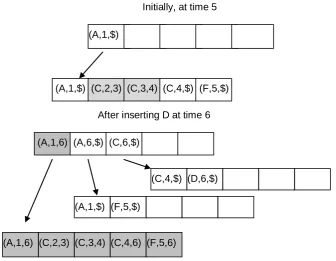
Figure 1 shows a possible instance of a partially persistent B-tree, and a simple scenario. At time 5 (upper part of the figure), the tree consists of two nodes, the root and one leaf, which contains all the data records. The figure shows that key A was inserted at time 1, key C was inserted at time 2 and was subsequently modified at times 3 and 4, and key F was inserted at time 5. Then, at time 6, key D is to be inserted. This insertion causes an overflow of the single leaf. Two new leaves are then created and the old leaf becomes inactive (all the inactive records appear shaded). The index record of the root, which points to the inactive leaf, also becomes inactive (shaded). The set of live records of the old leaf is sorted by key, is divided into two halves and each of these halves is copied to one of the two new leaves. Two new index records are created in the root. Their start value is the time at which the pointed leaves were created, i.e. time 6. To delete a record, we set its end-value to the current time instance and then count the remaining live records of the leaf. If they are too few, we may borrow some live records from a neighbour leaf, and create one or two new leaves.
The fact that one or two leaves may be created requires some brief discussion. In the scenario of Figure 1, the rebalanced leaf contains less than 5 active records. Since however 5 records fit into one leaf, one would expect that only one new leaf is needed. Instead, one can see that we have created two new leaves. Appropriate explanation for this decision is now justified by the following: In general, the number of new leaves created is dictated by our need to create “stable” leaves that will not be rebalanced soon. As an example, let us set to B the capacity of each node of the persistent tree. If the leaf being rebalanced contains B active records, then we can move all the active records to a new leaf but this leaf will immediately be rebalanced if a new insertion occurs inside it. The general rule is that we create one or two
“stable” leaves, each of them requiring Θ(B) updates (insertions or deletions)
in order to be rebalanced again. After a deletion, we count the number of active records inside the node containing the “deleted” record. If the number is smaller than a threshold, then we may transfer some active records to that node, from a neighboring node, or merge this node with a neighboring node, and create one or two stable nodes. It is easy to see that creating stable nodes is not a difficult task (further details can be found in [2] and [13]). Thus, partially persistent B-trees have the following property, which is important for our solutions.
In order to achieve Property 2, the minimum number of active records
inside a node must be Θ(B) otherwise, a node will have to be merged before it
“experiences” Θ(B) “delete” operations. Assuming for example that the
minimum number is 4 then, by merging two nodes, we create one node with at least 8 active records. This node can then experience 4 deletion operations before it has to be merged again. The fact that the minimum number of records is set to Θ(B), leads to Property 3, which is also important for our solutions.
Property 3: If we navigate into the persistent structure at time instance t,
each node we access has Θ(B) records, valid at this instance.
Fig. 1. A simple scenario of a partially persistent B-tree. The ptr-field for each record is visualized through an arrow pointing to the level below. The fields key, start and end, are shown in the same order. The shaded records are inactive and the remainder are active.
Let us now briefly describe the navigation inside a partially persistent B-tree. To search for a key K that is valid at time t, we start from the root. We ignore the records with start values greater than t and the records with end
values less than t. From the remaining records we choose the one with
greatest key value, less than or equal to K; if there are several such records,
we choose that one with the greatest start value. We follow the pointer to the
next level and we then apply the same procedure at this level. Note that this process introduces a unique path towards the leaf level, where a leaf is
(A,1,$)
(A,1,$)
Initially, at time 5
After inserting D at time 6 (A,1,$) (C,2,3) (C,3,4) (C,4,$) (F,5,$)
(A,1,6) (A,6,$) (C,6,$)
(A,1,6) (C,2,3) (C,3,4) (C,4,6) (F,5,6) (F,5,$)
accessed. The record will be found in the leaf if it really exists; otherwise, there was no record with key K valid at time t. Searching for example for element F at time instance 5 of Figure 1, we shall ignore records (A, 6, $) and (C, 6, $) because they were created after time instance 5. If, on the other hand, we search for element D at time 6, we shall ignore record (A, 1, 6) in the root of the structure, because this record was “deleted” at time 6. From the remaining records, we choose (C, 6, $) and we then follow the pointer indicated by this record.
The space consumption of optimal partially persistent B-trees is O(m/B)
blocks (where m is the total number of updates) and updates can be
performed in a O(logB(m/B)) worst case time. In the amortized case, the
update time is constant (see [2], [13]).
4. Static Indexing
We consider a grid on our 2-d map. In the static indexing we assume that the horizontal and vertical lines of the grid are determined in advance and they do not move during the monitoring period. Hence, the 2-d map is divided into static cells. Each incoming message is a tuple (Oid, Cid, t), where Oid is the id
of the object that sent the message, Cid is the id of the cell that contains Oid,
and t is the time at which the message was sent. For simplicity, we assume that each object can determine its current cell, i.e., it has some computational power. If this is not the case, the current cell can easily be determined by the system, with a simple calculation. The objects inside each cell are indexed by
a partially persistent B-tree. Each time an object leaves a cell C2 and enters
another cell C1, its record, which is located in C2 is set to inactive, by replacing
the value $ of its end field by the time at which the object sent the message.
Next, a new record for this object is inserted into the persistent B-tree of C1.
Its start value is set equal to the time at which the message was sent, and its
end value is set to $. This approach is described in Subsections 4.1 and 4.2.
4.1 Data Structures
For each cell Ci of the grid, we maintain in secondary memory a partially
persistent B-tree, called PBCi. In primary memory we maintain the following
data structures:
For each cell Ci of the grid, we maintain an indexing structure called
active_PBCi. Let Ci be a cell. PBCi contains both active and inactive
nodes. The active_PBCi is the tree defined by the active nodes of PBCi
and the pointers that connect these active nodes. For every leaf V of the
active_PBCi, there is a leaf X in PBCi which satisfies the following
property: At the time V was created, X was also created to be identical to
V. We call X,image of V, and we store into V a pointer towards X.
A table A containing the tracked objects. Suppose that we receive a
message from object i. Then entry A[i] contains the current cell of the object.
4.2 Algorithm to Handle Incoming Messages
Suppose we receive a message (Oi, Ck, t). The algorithm for the processing of
this message follows, and the result of the algorithm is visualized in Figure 2.
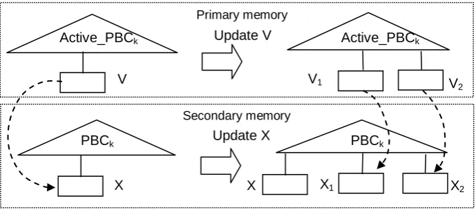
Fig. 2. Deactivating leaf V in cell Ck, leads to updating its image leaf X on the disk
Step 1: We go to A[i] and find the current cell of Oi. Let Cj be that cell. If Ck =
Cj, we do nothing. Otherwise we store Ck, in A[i] and proceed to Step 2.
Step 2: We find the appropriate leaf V in the active_PBCk and insert into it the
new tuple. If V is not full, we are done. If V is full we may have either to split, or merge V with a neighboring leaf. In either case, one or two new
Active_PBCk
V
Primary memory
Update V Active_PBCk
V1 V2
PBCk
X
Secondary memory
Update X PBC
k
X1 X2
leaves must be created. Figure 2 shows the actions of Step 2, in the case at which V is split into two leaves, named V1 and V2. We execute the
insertion algorithm of the partially persistent B-tree on the active_PBCk,
with one difference: we throw away all the inactive nodes. For example, in Figure 2, leaf V is thrown away when the algorithm finishes. By following the pointer from V we reach X, the image of V. We then update X, to be
identical to V. Next, we proceed with the insertion algorithm on PBCk, and
we create the image leaf of each new leaf created by the insertion algorithm in the active_PBCk (X1 is the image leaf of V1 and X2 is the
image leaf of V2). We connect each new leaf in primary memory, with its
image leaf in secondary memory.
Step 3: In the active_PBCj, we find the leaf that contains the tuple of Oi. We
execute the deletion algorithm of the partially persistent B-tree on the
active_PBCj, in order to delete the tuple of Oi, in the same way we
executed the insertion algorithm in Step 2.
4.3 Analysis of the Solution
Lemma 1: If W is the total number of messages received by the system, then
the approach of this section stores these messages in O(W/B) message
storing I/Os, i.e., Property 1 holds:
Proof: When a leaf in primary memory becomes inactive, all its records are stored in the image leaf. According to the algorithm of the partially persistent B-tree, every leaf of an active_PB remains active until Θ(B) insertions or “deletions” (i.e., record deactivations) occur (due to Property 2). Each insertion or “deletion” corresponds to a message that has not been stored.
Thus, when a leaf is deactivated, Θ(B) new messages are stored in
secondary memory. By new, we mean messages that have not been stored in
secondary memory earlier. As a result, in order to store all the W messages, we need O(W/B) I/Os.
Lemma 2: Let S1 be the amount of primary memory occupied by active
nodes. Then, S1 is Θ(N).
Proof: Let u be an active node of an active_PB. Then u contains active records. We know that, in every node, the total number of records is at most B and the number of active records is Θ(B) (due to Property 3). Since the number of active records stored in all the active leaves of active_PBs is N
(equal to the number of tracked objects), we conclude that the total number of
records stored in all the active leaves of active_PBs is Θ(N). Adding the space
occupied by the internal nodes, the total space is multiplied by a constant less than 2. Therefore we conclude that the total space consumed by the active_PBs is Θ(N).
Due to this, the definition of active_PBs has to be revised as follows: If Ci is a
cell of the grid then the active_PBCi contains all the active nodes of PBCi plus
the inactive nodes inside the I/O list.
To determine the amount of main memory consumed by the approach of
this section, we notice that this amount is equal to the space (S1) occupied by
the active nodes, plus the space occupied by the deactivated nodes inside the
I/O list. Let S2 be the amount of primary memory occupied by nodes
deactivated during one time-period. As Lemma 3 states, the space occupied
by nodes deactivated during one time-period, is O(N).
Lemma 3: The amount of primary memory occupied by the nodes deactivated during one time-period is O(N).
Proof: We attach a counter on every leaf of the active_PBs. When a new leaf is created, its counter is set to 0. Each incoming message may produce an update to at most two leaves, the leaf that contained the object, and the leaf that contains the object currently. If an update occurs inside a leaf, the
counter of the leaf is increased by 1. Assume now that the N messages sent
within the same time period have been processed (the I/O list is empty), and
let X be the number of times that any counter has been increased by 1. Since
every message increases by 1 at most two counters, it is obvious that X ≤ 2N.
From these X times that a counter has been increased, only X / Θ(B) times have led to a rebalancing operation, because of Property 2. Thus, the total
number of rebalancing operations among the leaves of the active_PB’s is
O(N/B). The nodes involved in these rebalancing operations are those that became inactive during the time period and, since each of them occupies O(B) space, we conclude that the total space occupied by them in primary
memory is O(N).
All we now need is to make sure that the hardware is capable of performing all the I/Os created during a time period, before the next time period ends (otherwise the I/O list would grow indefinitely, leading to a vast consumption
of primary memory). Thus R, the maximum number of I/Os the hardware can
perform, must be big enough. This is logical, because even if the number of I/Os caused by our solution is asymptotically optimal, we still need hardware that can handle this amount of I/Os, otherwise the solution will not work. This
is why parameter R and the I/O list have been included in the solution, i.e. in
order to indicate the hardware requirements. Apart from that, they add nothing to the solution. From Lemmas 2 and 3, it follows that, as long as R = O(N/(T*B)) we conclude that M = S1+S2= Θ(N).
From the analysis of partially persistent B-trees ([2], [13]), it can easily be
deduced that the secondary memory used is O(W/B) blocks.
4.4 Spatiotemporal Range Predicates
processing of such a predicate by using a grid and a persistent structure for each cell of the grid was discussed in [9]. Here, we use the same solution, except from the fact that now we have to additionally search in primary memory.
Consider the predicate (S1, T1), where S1 is the cell C1 and T1 is the time
instance t1. Let F(C1, t1) be the set of objects satisfying the predicate (C1, t1).
We then have to look in both the active_PBC1 and in PBC1, in order to retrieve
all the records that correspond to objects that were inside cell C1 at time
instance t1. Let D1 and D2 be the set of objects corresponding to the records
retrieved from active_PBC1 and PBC1, respectively. Then F(C1, t1) = D1 U D2.
Now assume that the temporal constraint T1 is the time interval [t1, t2]. To
retrieve all the records corresponding to the objects that were inside the cell for a time instance in [t1, t2], we have to look again in both the active_PBC1
and in PBC1. First, we access all the leaves that were active at time t1. Then
we can follow the history from time t1 up to time t2. The ability to follow the
history is justified as follows: When one or two leaves of the index structure become inactive, either one or two new leaves are created. When a leaf L
becomes inactive we store into it a pointer to the newly born leaf. If two new leaves are created, we store two pointers into L. Following the pointers we retrieve all leaves that were valid at some time instance during the interval [t1,
t2]. These leaves contain the output of the query.
In [9] it is proved that, we can evaluate the spatiotemporal predicate (C1,
T1), by sparing at most O(logBWC1 + F(C1, T1)/B)) I/Os, where WC1 is the
number of updates occurred inside cell C1.
5. Dynamic Indexing
The approach of Section 4 may not be the best if we are interested in nearest
and k-nearest neighbour predicates. Such a predicate is a pair (Q, T), where
Q is a point on the map and T can be either a time instance or a time interval.
The output is the nearest object (or the k-nearest objects) to Q, at the time instance T or during the time interval T. The reason for the potential inefficiency of static indexing in this case is the following: If the query point is on an empty cell, we have to start searching the neighbouring cells. That is, in case of a sparse traffic, we will end up consuming too much time (one I/O per cell) discovering empty cells. To face the disadvantages of the grid approach, we need a more dynamic partitioning of the d space. Thus, we divide our 2-d space by using only vertical lines. The area between two consecutive vertical lines is called slab, thus each slab is determined by its left and right border in the x-coordinate. Contrary to grid cells, slabs can easily be indexed in a way that their x-range is not static, i.e., the vertical lines that define slabs can “move” during the monitoring period. The reason is that by moving a line we have to update only 2 slabs whereas in Section 4, if we move a vertical line, we will have to update many cells. The reason for moving a line is to
follows:If d is a constant, it is said that the slabs are equally balanced if the most populated slab has at most d times the number of objects of the least populated slab.
Maintaining equally balanced slabs, we know that the slab containing the query point will always contain an object that is “fairly close” to the query point, and can be used as a starting-point in order to find the nearest neighbor. After finding a starting point, we are able to bound the search area for the nearest neighbor, by searching for objects that are closer to the query point than the starting-point. Each time we find a new nearest neighbor, we bound further the search area.
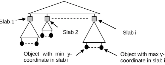
We index the objects inside each slab, by their y-coordinate. Assuming that the slabs are thin enough, the y-coordinate suffices to track the objects inside each slab with a satisfactory precision. If follows, that we can track the current position of the objects by a two-level indexing structure (Figure 3). The upper level is an index for the slabs. Each leaf of the upper level corresponds to a slab and it is connected to an indexing structure of the lower level, which stores the objects inside the slab, by their y-coordinate. If we want to track the past positions of the objects also, we have to make this two level indexing structure partially persistent.
Fig. 3. The two-level partially persistent indexing structure.
To make things easier during the description of the approach we assume, as in Section 4, that when a message storing I/O is needed, it is performed immediately. In Subsection 5.4, we add an I/O list to the solution i.e., when a message storing I/O is needed, it is inserted into the I/O list that works in FIFO order. Finally, in Subsection 5.5, we explore the efficiency of the approach for the handling of nearest and k-nearest queries.
Slab 1
Slab 2 Slab i
Object with min y-coordinate in slab i
5.1 Data Structures
In secondary memory we maintain the two-level persistent indexing structure described above. We call this structure, slab_index. The upper part is a persistent B-tree, and the same also holds for each tree of the lower part.
In primary memory we maintain an indexing structure created by the active nodes of the slab_index. We call this structure active_slab_index. In primary
memory we also maintain a table A, to store the objects. Position i of A stores
a pointer to the record of object i, in the active_slab_index.
5.2 Splitting and Merging Slabs
A slab has to merge with another slab, if its objects reduce to NL -1 and it has
to split if its objects increase to NH+1. Parameters NL and NH are going to be
determined later on. A slab that has more than ΝΗ objects is called big,
whereas a slab that has less than NL objects is called small. A slab that is
neither big nor small is called normal. The split and merge operations are incremental i.e., they are completed through small steps, where each such step costs a constant amount of time. Incremental split/merge steps are performed each time we receive a message from an object that is either inside or entered or left one of the involved slabs.
The incremental merge operation works as follows: Assume that slab Si
has NL-1 objects. Let TRi be the tree of the lower level of the
active_slab_index that corresponds to Si. Let Sj be the slab that is going to be
merged with Si, and TRj be the lower level tree that corresponds to Sj. TRi and
TRj have the same parent, u. Our objective is to merge trees TRi and TRj,
incrementally. The merging procedure is straightforward. In particular, every incremental step merges O(1) objects from each tree, according to their y-coordinate, starting from the leftmost leaf of each tree. Each merged record is inserted into tree TRk, which is going to replace trees TRi and TRj.
Incremental merge steps are performed each time we receive a message from an object that is either inside or entered or left one of the two merging slabs.
Suppose now that the number of objects of slab Sk increased to NH+1, i.e.
we have to split Sk. Again, the split is incremental. Each incremental step,
processes O(1) records of the lower level tree, TRk, corresponding to Sk, and
inserts them into a temporary balanced binary search tree, according to their
x-coordinate. When all the records of Tk are inserted into the temporary tree,
we start creating the two new slabs that are going to replace Sk. We
incrementally traverse the leaves of the temporary tree (O(1) records per incremental step) from left to right. The left half data records enter the new lower level tree TRk1 that corresponds to the new slab Sk1. The right half data
records enter the new lower level tree TRk2 that corresponds to the new slab
is split into two, and each new upper level leaf is connected with one new lower level tree.
During the incremental merge, an object Oi may have a valid record in at
most two trees. The first record (the one pointed by the pointer in position A[i]) is inside a leaf (L1) of a lower level tree (T1) corresponding to an existing slab.
The second record is inside a leaf (L2) of a tree under creation (T2). If a new
message arrives from Object Oi, both leaves must be updated. We reach the
record of Oi in L2 by storing to the record of Oi in L1, a pointer to L2.
It remains to give the algorithm that triggers these split/merge operations. This algorithm, which is called overall algorithm, guarantees that there is an upper and a lower bound to the number of objects inside each slab. The problem that needs to be solved is the following: Assume that a slab Si has
NL-1 objects, therefore it must merge with another slab. However, both
neighboring (to Si) slabs are under an incremental split/merge operation.
Then, Si must wait for at least one of these split/merge operations to finish.
The overall algorithm must guarantee that Si will not wait forever and
furthermore, all slabs are “equally balanced”. The main idea of the overall algorithm is the introduction of critical slabs. If Si is found to be small and all
the neighbouring to Si slabs are under split/merge operations, then Si
becomes critical. From that point, and as long as Si is critical, when an update
occurs inside Si, an incremental step is performed for each neighbouring (to
Si) split/merge operation. The overall algorithm follows.
Begin (overall algorithm)
We set NH = 10NL and we also set for each incremental step, to process at
least 65 active records. Suppose that we perform an update inside a slab Si.
Step 1: If Si is already under a split/merge operation, we perform an
incremental step for this split/merge operation.
Step 2: If Si is found to be big (i.e. if it has more than NH objects), a split
operation starts for Si.
Step 3: If Si is critical, then an incremental step is performed for each
neighbouring (to Si) split/merge operation.
Step 4: If Si is found to be small (i.e. it has less than NL objects), we have to
find another slab to merge it with Si. If there is a slab Sj next to Si, such
that Sj is not under a split/merge operation, then we merge Si with Sj.
Otherwise, Si becomes “critical”.
Step 5: If we have just executed the last incremental step for a merge operation and the resulting slab is big, (see Lemma 4) then the resulting slab immediately starts a split operation.
Step 6: If we have just executed the last incremental step for a merge operation and the resulting slab is normal, the resulting slab starts a merge operation with its neighbour that first became critical (if it has critical neighbours).
Step 7: If we have just executed the last incremental step for a split operation, then (according to Lemma 5), the resulting slabs are normal. Each of the resulting slabs merges with its critical neighbour, if such a neighbour exists.
Since every incremental step is executed each time an update occurs, it follows that the objects inside a slab may increase by 1 in every incremental step, if the update that caused the incremental step was an insertion. Thus, if L is the number of objects inside a slab when the slab begins to split, then the number of incremental steps needed for the split is at most L/64 (since we process at least 65 objects per incremental step and one object can be added per incremental step). Similarly, if the total number of objects inside a pair of slabs that start to merge is L then the merge operation will need at most L/64 incremental steps.
Lemma 4: A merge operation always creates either a big or a normal slab. Proof: First of all, it is trivial to show that a merge operation may create a big slab. Assume that two slabs start to be merged. One of these slabs must be small, and the other must be non-big. We conclude that when the merge
operation starts, the maximum number of involved objects is 11NL -1. Even if,
during the merge operation, the two slabs experience only deletions, then the resulting slab will have more than 11NL – 1 – (11NL – 1)/64> 10NL objects,
i.e., it will be big.
We are now going to prove that a merge operation does not create a small slab. In order to do that, we are going to determine the minimum number of objects involved in a merge operation, according to the overall algorithm.
Assume thus that a slab Si becomes small, but all the neighbouring slabs are
under a merge operation. Thus, Si becomes critical, and at the time one of
these merge operation ends, Si has at least NL-11NL/64 elements objects
(each merge operation involves at most 11NL objects). Let Sj be the slab that
results from this merge operation. Sj is then merged with its neighbouring slab
that first became critical, and this neighbouring slab may not be Si. Thus, Si
remains critical until this new merge operation ends, and let Sk be the bucket
that results from this merge operation. According to the overall algorithm, Sk
will be merged with Si, because if Sk has two critical neighbors, Si is the one
that first became critical. When Sk starts to be merged with Si, Si has at least
NL-22NL/64 objects. Thus the minimum number of objects inside a slab, when
the slab starts a merge operation is NL-22NL/64. We conclude that the
minimum number of objects involved in a merge operation, when the merge operation starts is 2(NL-22NL/64) objects. Even if during the merge operation,
all the updates that occur inside the two slabs are deletions, it follows that the resulting slab has at least 2(NL-22NL/64) - 2(NL-22NL/64)/64>2NL-3NL/8>NL
objects. Therefore, the resulting slab is not small.
Lemma 5. A split operation always creates normal slabs.
Proof: First of all we have to determine the maximum number of elements inside a slab, when this slab starts to be split. If slab Si drops to NL-1 objects,
it starts to merge with a slab Sj, which is not under a split process. When the
incremental merging process completes, the resulting slab has at most 11NL+11NL/64 objects (if Sj had NH objects and only insertions occurred
during the merge operation). Thus, the maximum number of elements inside a slab, when this slab starts to be split is 11NL+11NL/64.
the split operation), then at the time the split ends, the number of objects may increase to 11NL+11NL/64 +(11NL+11NL/64)/64< 12NL which means that each
new slab has at most 6NL objects (i.e., it is not big)
Let us now show that a split operation creates non-small slabs. Each split starts with more than 10NL+1 objects. If only deletions occur during the split
operation, the resulting slabs will have more than (10NL-10NL/64)/2 >4NL
elements.
Lemma 6. The slabs are “equally balanced”.
Proof: From Lemmas 4 and 5 it follows that the minimum number of objects inside a slab is NL-22NL/64, whereas the maximum number is less than 12NL.
This means that the maximum number is less than is 19 times greater than the minimum number and according to Definition 3, Lemma 6 follows
We have not set the value of NL. From a theoretical point of view, any value
is fine. From a practical point of view however, a very small value would create too thin slabs, leading to many split/merge operations between slabs, which will increase the number of I/Os (although they will still be asymptotically optimal). On the other hand, a big value would create too thick slabs, and this fact will have a negative effect on the efficiency of the system
for answering queries. Thus, the value of NL should be determined according
to the above guidelines, through experiments.
A technical detail still remains in the dark. When a split (merge) operation completes, the lower level tree (trees) corresponding to old slab (slabs) becomes inactive. For each object inside the leaves of such (i.e., inactive) trees, we update the corresponding pointer in table A, to point to the correct position, which is a leaf of the new tree. The space occupied by the nodes of this tree cannot be released immediately. Some leaves of the tree may not be identical to their image leaves in secondary memory. These image leaves
must be updated. This task is called cleaning procedure, and it is charged on
the slabs created by the split/merge procedure. It is easy to see that the I/Os caused by the cleaning procedure do not asymptotically change the number
of message storing I/Os, since a slab being cleaned, has experienced O(NL)
updates, and the number of message storing I/Os needed to clean it is O(NL/B).
5.3 Algorithm to Handle Incoming Messages.
Suppose we receive a message (Ok, x_value, y-value, t).
Step 1. We search the active_slab_index in order to find the slab (which is a leaf of the upper level) containing that x_value. Let Si be that slab. We
search table A and find the record of the object. Moving upwards in the lower level tree containing that record, we reach its root, and therefore we find the previous slab of the record. Let Sj be the previous slab.
Step 2. If i=j, we reach the current record of Ok and update its y-coordinate.
proceed to the update algorithm of the persistent structure. As in Section 4, if an active leaf becomes inactive we update its image leaf in the slab_index, and if a new active leaf is created, we create its image-leaf in the slab_index. If the record of an object is copied (as a result of the rebalancing of a leaf) to a new leaf, we update the pointer in A for that object. In particular, we store in A[k] a pointer pointing to the new record of object Ok.
Step 3. If i≠j, we delete (deactivate) the current record of the object in Si and
we insert a new record for that object in Sj. The insertion or deletion is
performed as in step 2.
Step 4. We update Si and Sj according to the overall algorithm.
5.4 Analysis of the Solution
Assuming that no slab is ever split or merged with another one, it can be easily derived using the arguments of Section 4 that the total number of
message storing I/Os is O(W/B), i.e. property 1 holds. However, the existence
of split/merge operations between slabs complicates things, because it is not now clear that Property 1 holds. All we need to show is that the total number of message storing I/Os because of the split/merge operations between slabs is also O(W/B). This is proved by Lemma 7.
Lemma 7: The total number of message storing I/Os created by the
incremental split/merge operations between slabs is O(W/B).
Proof. We attach a counter on every slab. When a new slab is created, its counter is 0. If an update occurs inside a slab, the counter of the slab is increased by one. Therefore, each incoming message may produce an
update into at most two slabs. After the W messages have been applied, let X
be the number of times that any counter increased by 1. It is obvious that X ≤
2W. From these X times that a counter was increased, only X/Θ(NL)
split/merge operations occurred, because each split/merge operation “costs”
Ο(NL) incoming messages (since each incoming message triggers an
incremental split/merge step and each such step processes a constant number of data records). Thus, the received messages generate at most O(W/NL) split/merge operations. Each split/merge operation creates Θ(NL/B)
message storing I/Os. We conclude that the total number of message storing
I/Os because of the incremental split/merge operations is
O(W/NL)*Θ(NL/B)=O(W/B).
The space occupied by our structures in secondary memory is O(W/B)
blocks, as in Section 4. This can be easily derived by the analysis of partially persistent B-trees (see [2], [13]). Concerning the space occupied by the active nodes in primary memory, Lemma 2 continues to be satisfied and as a result,
this amount of space is O(N). Assuming that each I/O is performed
immediately, no additional amount of primary memory is needed. Otherwise,
make sure that the space occupied by inactive nodes corresponding to pending I/Os (inside the I/O list), is also O(N). Lemma 3 continues to hold and, as a result, we conclude that the amount of primary memory used remains O(N), as long as R = O(N/(T*B)).
5.5 Nearest and k-nearest Neighbor Queries
As mentioned in Section 2, by indexing the space in a dynamic way we are
able to efficiently process Spatio-temporal nearest (k-nearest) neighbor
predicates. Suppose we have to process the nearest neighbor predicate ((x,
y), T), where x, y are the x- and y-coordinates of the query point and T is a temporal constraint (time instance or time interval).
Assume first that T is a time instance t. We find the slab containing (x, y) at
time t, by searching the slab_index and the active_slab_index, using x and t
as keys. When we reach the leaf of the upper level that is connected to the slab of interest, we proceed to the lower level tree. We search the lower level tree using y and t as keys. We extract O(B) records valid at time t and, from
these records, we choose the closest to the query point. Let Ok be that object.
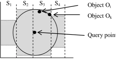
Figure 4 shows a possible scenario. Observe that Ok, which is found to be the
closest object to the query-point inside the slab that contains the query-point, is not actually the closest object. Indeed, it is Oi which is is closer. This “error”,
occurred because we use only the y-coordinate to index all the objects inside the same slab and, with respect to the y-coordinate, Ok is closer than Oi to the
query point. Object Ok may not be the closest to the query point, but it can be
used as a “pruning tool”. In particular, we now know that there is no reason to search for the nearest object outside the circle in Figure 4. This circle enables us to search inside the gray area, because this is the best we can do according to our indexing structures. (We can afford to efficiently search between two y-coordinates inside each slab.)
Fig. 4. Ok is not the closest object to the query point inside S3, although it was
retrieved as such by searching inside S3
Observe that Oi, in Figure 4, may not in fact be the object closest to the
query point, because slab S2 may contain an object that is even closer. A
search in S2 will reveal the one closest. The advantage of the above
described strategy is that we always find an initial object, which can be used
S1 S2 S3 S4
Object Ok
Object Oi
as a pruning tool (Ok in Figure 4), because all slabs have objects. This
advantage may prove valuable in terms of time efficiency, especially in cases where the number of objects is small or in cases where the movement of the objects tend to form areas of very sparse traffic.
If the time constraint T is a time interval [t1, t2], things are more
complicated. Here is a general description. During time, we keep the “history” of the leaves by using pointers as explained in Subsection 4.4. We find the
nearest neighbour to the query point, at time t1, as described in the previous
paragraph. Suppose that the nearest neighbour at time t1 is object Oj (see
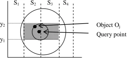
Figure 5). Then, the area of interest contains the slabs intersected by the circle (i.e., S2 and S3, between y1 and y2). For each slab, we must search in
the interval (t1, t2], for a potential new nearest neighbour. All we need to do is
to “follow the time”. This can easily be achieved by the use of pointers that lead, with respect to time, to the descendants of each leaf. Since at most two leaves can be created by a leaf rebalance, it follows that we can move forward in time, by storing two pointers in each leaf. We start from each leaf that contains elements in the gray area at time t1, and follow the pointers
leading to the future, until we reach leaves created after t2. In each leaf we
access, we search for a potential new nearest neighbor. Every time we find a new nearest neighbor, we update the slabs and areas of interest.
Fig. 5. The dark-shaded area is the area of interest created by Oj, which is the nearest neighbour of the query point at time t1. Accessing the leaves that correspond to the
gray area at time t1, and moving forward in time until we reach t2, we manage to
retrieve the final (and truly) nearest neighbour.
We can use this solution to answer k-nearest neighbor queries as well. The only difference is that initially, we retrieve the k-nearest neighbors from the slab containing the query point. Then, the intersecting slabs and the ranges of interest in each slab, are determined via the k-th nearest neighbor after each I/O.
6. Dealing with the Rebalancing I/Os
In Sections 4 and 5 we assumed that no rebalancing I/Os occur, and this assumption is not realistic. Indeed a message storing I/O may trigger a non-constant number of rebalancing I/Os. However, in case that the tracking
S1 S2 S3 S4
Object Oj
Query point y1
period is longer than P (which is a realistic assumption), the amortized number of rebalancing I/Os per message storing I/O is constant. This is because the amortized update cost of the partially persistent B-tree is constant. As a consequence, Property 1 holds for the solutions of Sections 4 and 5, even if we take the rebalancing I/Os into account.
For a strictly theoretical solution (without the above realistic assumption), it suffices to guarantee that after a message storing I/O, O(1) rebalancing I/Os
in the worst case may occur. Thus, to solve the problem, we need a partially persistent B-tree with constant worst case update time. Such a structure was recently presented (see [7]), and by adapting it in Sections 4 and 5 as our basic tree structure, we achieve O(1) rebalancing I/Os per message storing I/O, in the worst case.
7. Conclusions and future work
In this paper we studied the problem of storing the past and present positions of moving objects and proposed theoretical solutions for storing the messages sent by the moving objects in a way that guarantees that the number of the involved I/Os is asymptotically optimal. This way, we managed to face the bottleneck caused by the large number of messages that must be taken into account in order to update the involved indexing structures.
In particular, we presented solutions that require O(W/B) I/Os for storing
the messages (where W is the total number of messages and B is the number
of messages that fit into a disk block) and require O(N) primary memory
(where N is the number of tracked objects). Furthermore, our solutions allow
for the efficient processing of interesting queries. To show this, we focused on the processing of well-known spatiotemporal range predicates and nearest neighbor predicates, which have been studied thoroughly.
Exploring the efficiency of our solutions, in order to answer other interesting queries, is a promising field for future work. New queries emerge daily from real life demands and, for each such query, a solution based on the techniques we presented in this paper may turn out to be useful.
Also, the implementation of our techniques is another interesting piece of research. However, a strict implementation of the proposed solutions is not a very good idea. Such an implementation should definitely incorporate ideas from other implementation oriented research efforts in order for practical efficiency worthy of investigation, to be achieved.
References
1 Aggarwal, A., Vitter, J. S.: The input/output complexity of sorting and related problems. Communications of the ACM, Volume 31, Issue 9, 1116-1127. (1988) 2 Becker, B., Gschwind, S., Ohler, T., Seeger, B., Widmayer, P.: An asymptotically
optimal multiversion B-tree. The VLDB Journal, Volume 5, Issue 4, 264-275. (1996)
3 Biveinis, L., Saltenis, S., Jensen C. S.: Main memory operation buffering for efficient R-tree update. In the Proceedings of the 33rd international conference on Very large data bases (VLDB), ACM, Vienna, Austria, 591-602. (2007) 4 Cheng, R., Xia, Y., Prabhakar, S., Shah, R.: Change Tolerant Indexing for
Constantly Evolving Data. In the Proceedings of the 21st International Conference on Data Engineering (ICDE), IEEE Computer Society press, Tokyo, Japan, 391-402. (2005)
5 Driscoll, J. R., Sarnak, N., Sleator, D. D., and Tarjan, R. E.: Making Data Structures Persistent. Journal of Computer and System Sciences, Volume 38 Issue 1, 86-124. (1989)
6 Kwon, D., Lee, S., Lee, S.: Indexing the current positions of moving objects using the lazy update R-tree. In the Proceedings of the 3rd International Conference on Mobile Data Management (MDM), IEEE Computer Society, Singapore, 113-120. (2002)
7 Lagogiannis, G., Lorentzos, N.: Partially Persistent B-trees with Constant Worst Case Update Time. Computers and Electrical Engineering, Volume 38, Issue 2, 231-242. (2012)
8 Lagogiannis G., Lorentzos N. A., Sideridis A.B.: Indexing Moving Objects: A Real Time Approach. In the proceedings of the 3rd World Summit on the Knowledge Society (WSKS), Corfu, Greece, 421-426. (2010)
9 Lagogiannis, G., Lorentzos, N., Sioutas, S., Theodoridis, E.: A Time Efficient Indexing Scheme for Complex Spatiotemporal Retrieval. SIGMOD Record Volume 38, Issue 3, 11-16. (2009)
10 Lanka, S., Mays, E.: Fully Persistent B+-trees. In the Proceedings of the ACM SIGMOD Conference on Management of Data, Denver, USA, 426-435. (1991) 11 Lee, M. L., Hsu, W., Jensen, C. S., Cui, B., Teo, K. L.: Supporting Frequent
Updates in R-Trees: A Bottom-Up Approach. In the Proceedings of the 29th international conference on Very large data bases (VLDB), Berlin, Germany, 608-619. (2003)
12 Tung, H., Ryu K.: One update for all moving objects at a timestamp. In the Proceedings of the Sixth IEEE International Conference on Computer and Information Technology (CIT), IEEE Computer Society, Seoul, 6. (2006)
13 Varman, P. J., Verma, R. M.: An Efficient Multiversion Access Structure. IEEE Transactions on Knowledge and Data Engineering, Volume 9, Issue 3, 391-409. (1997)
George Lagogiannis is a Lecturer at the Agricultural University of Athens. He received his Diploma (1995) his M.Sc. (2000) and his Ph.D. (2003) in Computer Science, from the Department of Computer Engineering and Informatics of the Technical School of the University of Patras. His research interests are data structures and algorithms.
Nikos Lorentzos is a Professor at the Agricultural University of Athens. He has a first Degree in Mathematics (National and Kapodistrian University of Athens, 1975), a Master’s Degree in Computer Science (Queens College, CUNY, USA, 1981) and a Ph.D. Degree in Computer Science (Birkbeck College, University of London, 1988). His major research contribution is in Temporal, Spatial and Spatiotemporal Databases, and in the development of DSSs and Expert Systems in the forestry and agricultural domain.
Alexander B. Sideridis received a primary degree in Mathematics from the University of Athens, and an M.Sc. and Ph.D. from Brunel University. He is a Professor and Head of the Informatics Laboratory of the Agricultural University of Athens. His current research interests concern the design and implementation of Decision Support and Knowledge Based Systems