Bayesian Approaches For Modeling Variation

University of Pennsylvania

ScholarlyCommons

Publicly Accessible Penn Dissertations

2019

Bayesian Approaches For Modeling Variation

Gemma Elyse Moran

University of Pennsylvania, [email protected]

Follow this and additional works at:

https://repository.upenn.edu/edissertations

Part of the

Statistics and Probability Commons

This paper is posted at ScholarlyCommons.https://repository.upenn.edu/edissertations/3350 For more information, please [email protected].

Recommended Citation

Bayesian Approaches For Modeling Variation

Abstract

A core focus of statistics is determining how much of the variation in data may be attributed to the signal of interest, and how much to noise. When the sources of variation are many and complex, a Bayesian approach to data analysis offers a number of advantages. In this thesis, we propose and implement new Bayesian methods for modeling variation in two general settings. The first setting is high-dimensional linear regression where the unknown error variance is also of interest. Here, we show that a commonly used class of conjugate shrinkage priors can lead to underestimation of the error variance. We then extend the Spike-and-Slab Lasso (SSL, Rockova and George, 2018) to the unknown variance case, using an alternative, independent prior

framework. This extended procedure outperforms both the fixed variance approach and alternative penalized likelihood methods on both simulated and real data.

For the second setting, we move from univariate response data where the predictors are known, to

multivariate response data in which potential predictors are unobserved. In this setting, we first consider the problem of biclustering, where a motivating example is to find subsets of genes which have similar expression in a subset of patients. For this task, we propose a new biclustering method called Spike-and-Slab Lasso Biclustering (SSLB). SSLB utilizes the SSL prior to find a doubly-sparse factorization of the data matrix via a fast EM algorithm. Applied to both a microarray dataset and a single-cell RNA-sequencing dataset, SSLB recovers biologically meaningful signal in the data.

The second problem we consider in this setting is nonlinear factor analysis. The goal here is to find low-dimensional, unobserved ``factors'' which drive the variation in the high-dimensional observed data in a potentially nonlinear fashion. For this purpose, we develop factor analysis BART (faBART), an MCMC algorithm which alternates sampling from the posterior of (a) the factors and (b) a functional approximation to the mapping from the factors to the data. The latter step utilizes Bayesian Additive Regression Trees (BART, Chipman et al., 2010). On a variety of simulation settings, we demonstrate that with only the observed data as the input, faBART is able to recover both the unobserved factors and the nonlinear mapping.

Degree Type

Dissertation

Degree Name

Doctor of Philosophy (PhD)

Graduate Group

Statistics

First Advisor

Edward I. George

Subject Categories

BAYESIAN APPROACHES FOR MODELING VARIATION

Gemma E. Moran

A DISSERTATION

in

Statistics

For the Graduate Group in Managerial Science and Applied Economics

Presented to the Faculties of the University of Pennsylvania

in

Partial Fulfillment of the Requirements for the

Degree of Doctor of Philosophy

2019

Supervisor of Dissertation

Edward I. George, Universal Furniture Professor, Professor of Statistics

Graduate Group Chairperson

Catherine M. Schrand, Celia Z. Moh Professor, Professor of Accounting

Dissertation Committee

Veronika Roˇckov´a, Assistant Professor of Econometrics and Statistics, Chicago Booth

Nancy R. Zhang, Professor of Statistics

BAYESIAN APPROACHES FOR MODELING VARIATION

c

COPYRIGHT

2019

Gemma Elyse Moran

This work is licensed under the

Creative Commons Attribution

NonCommercial-ShareAlike 3.0

License

To view a copy of this license, visit

Dedicated to my grandparents:

ACKNOWLEDGEMENT

First and foremost, I would like to thank my advisor, Ed George. Your incredible insight and

statistical intuition have been instrumental in shaping both this thesis and my development

as a statistician. Moreover, your boundless enthusiasm and encouragement always led me

to come away from meetings with a renewed positive outlook and energy, especially when I

was at my most stressed.

Thank you to my committee members: Veronika Roˇckov´a, Shane Jensen and Nancy Zhang.

Veronika - your tremendous work ethic and intellect have been an inspiration and I have

learnt so much from working with you over the course of my PhD. Shane - thank you

for being a fantastic teacher, for your wealth of knowledge of all things Bayesian and for

all your encouragement. Nancy - thank you for fostering my interest in both genomics

and dimensionality reduction - many of my current research interests were inspired from

attending your reading group.

Next, an enormous thank you to the Wharton Statistics Department. On my prospective

PhD visit from Australia five years ago, I was struck by the warmth and collegiality of the

department, a feature which has remained constant over my five years here. To the faculty

that I have been fortunate enough to have as teachers, thank you for your dedication and

helping me grow as a researcher and statistician. To the staff - thank you for all you do

to keep the department running smoothly, and for all your generous help, from reserving

classrooms for TA sessions, to navigating PhD forms and for always being there with kind

words and/or a donut.

To our PhD cohort - Raiden Hasegawa, Bikram Karmakar, Justin Khim and Linjun Zhang

- it has been a privilege to call you my classmates. I will always have fond memories of the

first year office where we would alternate doing our probability homework with playing putt

putt golf. To the Bayesian gang - Cecilia Balocchi and Sameer Deshpande - our reading

forward to future collaborations in the years to come! To the Statistics PhD students,

both present and graduated - thank you for all the laughs and great conversations, both

statistical and otherwise, over our daily lunches in the department, board game nights,

drinks at Cav’s and barbecues.

I feel so lucky to have so many amazing friends from all over the world. To my Philadelphia

friends - you have made my five years here enriching personally as well as intellectually.

Thank you especially to Lesley Meng, Cecilia Balocchi, Elica Dhundia McCarthy, Sameer

Deshpande, Kathy Li and Daniela Schmitt for always being there for me, from the stressful

times to the celebratory times, and everything in between. Finding balance during the PhD

was so important - thanks to the erstwhile running club: Justin Khim, Kathy Li, Lesley

Meng, Min Xu; the bowling crew: Justin Chiu, Colman Humphrey, Matt Olson; the bridge

club: Eric Baxter, Ashley Baker, Ling Lin; and the vegan food gang: Edward Chang and

Lesley Meng. To my Australian friends: true friendship is when it feels like just yesterday

since you’ve last seen each other, even if it has been a year - thank you.

To Eric Baxter - thank you for always being able to make me laugh, supporting me, being

there for me in tough times, and for all of our adventures, even when I forget to read contour

maps and plan a hike up an (almost) vertical mountain slope.

Finally, thank you to my family. As the quote goes - you have given me roots and wings.

Roots, to ground me and give me a sense of belonging and identity, and wings, to give me

the courage to go out in the wider world. Thank you especially to my parents: Gabrielle

and Paul, and Greg and Trish: even though I am on the other side of the world, it gives

me such strength knowing you are always there for me, just a call away. Nick - thank you

for being the best big brother. Margaret - thank you for being my “Philly Mum” - it has

been so wonderful to have had the opportunity to connect here and I am so grateful for all

your care, encouragement, and showing me this great city. Your equanimity, generosity and

In the week before submitting this thesis, my uncle Simon tragically passed away. Si

-thank you for being such a great uncle, from introducing me to my favorite sci-fi and

fantasy novels as a kid, to always having a witty response or joke for every situation, and

ABSTRACT

BAYESIAN APPROACHES FOR MODELING VARIATION

Gemma E. Moran

Edward I. George

A core focus of statistics is determining how much of the variation in data may be attributed

to the signal of interest, and how much to noise. When the sources of variation are many

and complex, a Bayesian approach to data analysis offers a number of advantages. In this

thesis, we propose and implement new Bayesian methods for modeling variation in two

general settings. The first setting is high-dimensional linear regression where the unknown

error variance is also of interest. Here, we show that a commonly used class of conjugate

shrinkage priors can lead to underestimation of the error variance. We then extend the

Spike-and-Slab Lasso (SSL, Roˇckov´a and George, 2018) to the unknown variance case,

using an alternative, independent prior framework. This extended procedure outperforms

both the fixed variance approach and alternative penalized likelihood methods on both

simulated and real data.

For the second setting, we move from univariate response data where the predictors are

known, to multivariate response data in which potential predictors are unobserved. In this

setting, we first consider the problem of biclustering, where a motivating example is to find

subsets of genes which have similar expression in a subset of patients. For this task, we

propose a new biclustering method called Spike-and-Slab Lasso Biclustering (SSLB). SSLB

utilizes the SSL prior to find a doubly-sparse factorization of the data matrix via a fast EM

algorithm. Applied to both a microarray dataset and a single-cell RNA-sequencing dataset,

SSLB recovers biologically meaningful signal in the data.

The second problem we consider in this setting is nonlinear factor analysis. The goal here

high-dimensional observed data in a potentially nonlinear fashion. For this purpose, we develop

factor analysis BART (faBART), an MCMC algorithm which alternates sampling from the

posterior of (a) the factors and (b) a functional approximation to the mapping from the

factors to the data. The latter step utilizes Bayesian Additive Regression Trees (BART,

Chipman et al., 2010). On a variety of simulation settings, we demonstrate that with only

the observed data as the input, faBART is able to recover both the unobserved factors and

TABLE OF CONTENTS

ACKNOWLEDGEMENT . . . iv

ABSTRACT . . . vii

LIST OF TABLES . . . xi

LIST OF ILLUSTRATIONS . . . xii

CHAPTER 1 : Introduction . . . 1

CHAPTER 2 : Variance Priors . . . 5

2.1 Introduction . . . 5

2.2 Invariance Criteria . . . 9

2.3 Bayesian Regression . . . 12

2.4 Connections with Penalized Likelihood Methods . . . 20

2.5 Global-Local Shrinkage . . . 22

2.6 Spike-and-Slab Lasso with Unknown Variance . . . 26

2.7 Protein Activity Data . . . 39

2.8 Conclusion . . . 42

2.9 Appendix . . . 43

CHAPTER 3 : Spike-and-Slab Lasso Biclustering . . . 47

3.1 Introduction . . . 47

3.2 Model . . . 54

3.3 Simulation Studies . . . 61

3.4 Breast Cancer Microarray Dataset . . . 65

3.5 Mouse Cortex and Hippocampus scRNA-seq Dataset . . . 70

3.7 Appendix . . . 77

CHAPTER 4 : Nonlinear Factor Analysis via BART . . . 91

4.1 Introduction . . . 91

4.2 Review of BART . . . 93

4.3 Related Work . . . 97

4.4 Nonlinear Factor Analysis via BART . . . 100

4.5 Identifiability . . . 105

4.6 Parametric Examples . . . 107

4.7 Visualization Examples . . . 111

4.8 Conclusion . . . 118

4.9 Appendix . . . 118

LIST OF TABLES

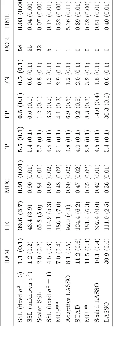
TABLE 1 : Comparison of penalized likelihood methods . . . 38

TABLE 2 : Estimates for number of biclusters . . . 64

LIST OF ILLUSTRATIONS

FIGURE 1 : Comparison of variance priors for ridge regression . . . 17

FIGURE 2 : SSL variance estimates . . . 39

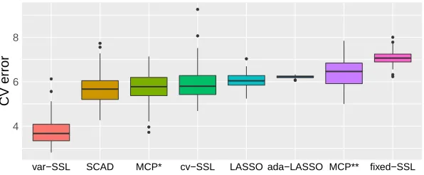
FIGURE 3 : Cross-validation error on the protein dataset . . . 41

FIGURE 4 : Illustration of rank-1 biclusters . . . 49

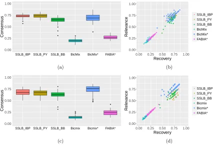
FIGURE 5 : Consensus, relevance and recovery scores . . . 63

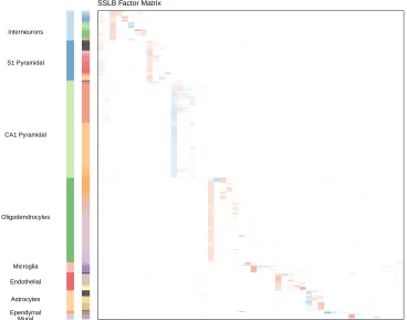
FIGURE 6 : Breast cancer dataset: SSLB results . . . 66

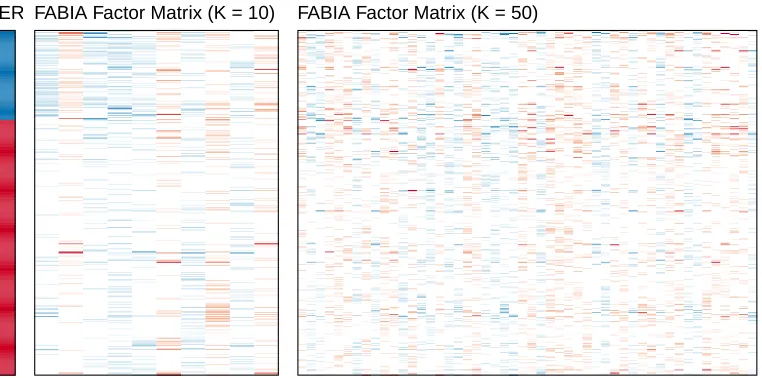
FIGURE 7 : Breast cancer dataset: FABIA results . . . 70

FIGURE 8 : Zeisel dataset: SSLB results . . . 72

FIGURE 9 : Zeisel dataset: BicMix results . . . 76

FIGURE 10 : Breast cancer dataset: comparison of raw and normalized data . . 83

FIGURE 11 : Breast cancer dataset: SSLB complete results . . . 84

FIGURE 12 : Breast cancer dataset: enrichment maps for SSLB genes . . . 85

FIGURE 13 : Zeisel dataset: SSLB complete results . . . 88

FIGURE 14 : Zeisel dataset: enrichment maps for genes in SSLB biclusters 1 & 2 89 FIGURE 15 : Zeisel dataset: enrichment maps for genes in SSLB bicluster 44 . . 90

FIGURE 16 : Illustrations for BART . . . 94

FIGURE 17 : Parametric Example 1: faBART results . . . 108

FIGURE 18 : Parametric Example 2: faBART and VAE results . . . 110

FIGURE 19 : Parametric Example 3: faBART and VAE results . . . 112

FIGURE 20 : Embeddings of Swiss-roll data . . . 115

FIGURE 21 : Example MNIST images . . . 117

FIGURE 22 : Embeddings of MNIST data . . . 117

CHAPTER 1 : Introduction

Statistics has been said to be the science of variation. A core problem of any statistical

analysis is determining how much of the observed variation in the data can be attributed to

the signal of interest, and how much to noise. Understanding and modeling these sources of

variation is crucial for both inferring the size and significance of the signal, and predicting

future realizations of the data.

In this thesis, we first consider the problem of high-dimensional linear regression where the

unknown noise variance is also of interest. We then move from this univariate response

setting where the predictors are known, to the multivariate response setting in which

po-tential predictors are unobserved. Although this lack of predictors presents an even greater

challenge, this multivariate setting also presents a tremendous opportunity to learn about

the covariation of the responses. In this setting, the covariation itself is often a signal of

interest; in gene expression data, for example, finding sets of responses which exhibit similar

behavior (that is, covary) can be an indication that these responses are driven by the same

underlying biological process.

To tackle the challenge of modeling variation in these settings, we adopt a Bayesian

perspec-tive. A Bayesian approach to modeling begins with specifying a data generating process, or

model. Within this model, the Bayesian paradigm allows for the coherent inclusion of

mul-tiple sources of variation which give rise to the observed data. In treating the parameters

of this model as themselves random, a Bayesian approach confers a number of advantages.

Firstly, it provides uncertainty quantification for the parameters via their posterior

distri-bution. Secondly, by treating the parameters as random instead of fixed, the parameters

are able to adapt to the data at hand. Finally, Bayesian analyses allow for the “borrowing

of strength” across multiple observations to ultimately yield parameter estimates which are

less susceptible to noise.

both the univariate linear regression setting, and the multiple response setting where no

predictors are observed.

In Chapter 2, we consider the problem of simultaneously estimating the regression

co-efficients and error variance in the high-dimensional Gaussian linear model. A common

Bayesian approach to modeling the error variance is to use a conjugate shrinkage prior

framework. Here, however, we show that these commonly used conjugate shrinkage

pri-ors can actually have detrimental consequences for error variance estimation. Such pripri-ors

are often motivated by the invariance argument of Jeffreys (1961). Revisiting this work,

however, we highlight a caveat that Jeffreys himself noticed; namely that biased estimators

can result from inducing dependence between parameters a priori. In a similar way, we

show that conjugate priors for linear regression, which induce prior dependence, can lead

to such underestimation in the Bayesian high-dimensional regression setting. Following

Jef-freys, we recommend as a remedy to treat regression coefficients and the error variance as

independent a priori.

In the latter half of Chapter 2, we then extend the Spike-and-Slab Lasso of Roˇckov´a and

George (2018) to the unknown variance case, using an independent prior framework. This

extended procedure outperforms both the fixed variance approach and alternative

penal-ized likelihood methods on simulated data. On the protein activity dataset of Clyde and

Parmigiani (1998), the Spike-and-Slab Lasso with unknown variance achieves lower

cross-validation error than alternative penalized likelihood methods, demonstrating the gains in

predictive accuracy afforded by simultaneous error variance estimation.

In the next part of this thesis, we move to the multivariate setting, where for each individual,

we observe many responses, or features. Unlike Chapter 2, however, we now do not observe

any potential predictors for these responses.

In Chapter 3, we consider the problem of finding small sets of individuals which covary

referred to as biclusters. In this way, biclustering methods differ from traditional clustering

methods, which find groups of individuals that are similar over their entire set of features.

Motivating applications for biclustering include genomics data, where the goal is to cluster

patients or samples by their gene expression profiles; and recommender systems, which seek

to group customers based on their product preferences. More precisely, biclusters of interest

are often assumed to manifest as rank-1 submatrices of the data matrix. This submatrix

detection problem can be viewed as a factor analysis problem in which both the factors and

loadings are sparse.

We propose a new biclustering method called Spike-and-Slab Lasso Biclustering (SSLB).

SSLB utilizes the Spike-and-Slab Lasso of Roˇckov´a and George (2018) to find a

doubly-sparse factorization of the data matrix. SSLB also incorporates an Indian Buffet Process

prior to automatically choose the number of biclusters. Many biclustering methods make

assumptions about the size of the latent biclusters, either assuming that the biclusters are

all of the same size, or that the biclusters are either very large or very small. In contrast,

SSLB can adapt to find biclusters which have a continuum of sizes. SSLB is implemented

via a fast Expectation-Maximization (EM) algorithm with a variational step. In a variety of

simulation settings, SSLB outperforms other biclustering methods. We apply SSLB to both

a microarray dataset and a single-cell RNA-sequencing dataset and highlight that SSLB

can recover biologically meaningful signal in the data.

In Chapter 4, we again consider the unsupervised multivariate response setting with the

goal of finding low-dimensional “factors” which drive the variation in the observed data.

Unlike in Chapter 3, however, we now relax the assumption that the observed data is

linearly related to the unobserved factors. This adds an additional layer of complexity to

the problem: we need to both estimate the unobserved factors, and the mapping between

the factors and observed data. To accomplish this task, we develop a Markov Chain Monte

Carlo (MCMC) algorithm which alternates between sampling from the posterior of the

Additive Regression Trees (BART), introduced by Chipman et al. (2010). We refer to

our method as Factor Analysis BART (faBART). On a variety of simulation settings, we

demonstrate that with only the observed data as the input, faBART is able to recover both

the unobserved factors and the nonlinear mapping. We then develop tempered faBART, a

modification of faBART which includes a tempering step to allow the algorithm to more

easily detect structure for data visualization. On two canonical datasets for visualization,

CHAPTER 2 : Variance Priors

2.1. Introduction

Consider the classical linear regression model

Y =Xβ+ε, ε∼Nn(0, σ2In) (2.1)

where Y ∈ _Rn _{is a vector of responses, X = [X}

1, . . . ,Xp] ∈ Rn×p is a fixed regression

matrix ofp potential predictors, β= (β1, . . . , βp)T ∈Rp is a vector of unknown regression

coefficients andε∈_Rn is the noise vector of independent normal random variables withσ2

as their unknown common variance.

Whenβis sparse so that most of its elements are zero or negligible, finding the non-negligible

elements ofβ, the so-called variable selection problem, is of particular importance. Whilst

this problem has been studied extensively from both frequentist and Bayesian perspectives,

much less attention has been given to the simultaneous estimation of the error varianceσ2_.

Accurate estimates of σ2 _{are important to discourage fitting the noise beyond the signal,}

thereby helping to mitigate overfitting of the data. Variance estimation is also essential in

uncertainty quantification for inference and prediction.

In the frequentist literature, the question of estimating the error variance in our setting

has begun to be addressed with papers including the scaled Lasso (Sun and Zhang, 2012)

and the square-root Lasso (Belloni et al., 2014). Contrastingly, in the Bayesian literature,

the error variance has been fairly straightforwardly estimated by including σ2 _{in prior}

specifications. Despite this conceptual simplicity, the majority of theoretical guarantees for

Bayesian procedures restrict attention to the case of known σ2_{, as there is not a generally}

agreed upon prior specification whenσ2 is unknown. More specifically, priors onβ and σ2

Adapted from a research article:

Moran, G. E., Roˇckov´a, V. and George, E. I. (2019) “Variance Prior Forms for High-Dimensional Bayesian

are typically introduced in one of two ways: either via a conjugate prior framework or via

an independence prior framework.

Conjugate priors have played a major role in regression analyses. The conjugate prior

framework for (2.1) begins with specifying a prior onβ that depends onσ2 as follows:

β|σ2 ∼N(0, σ2V), (2.2)

where V may be fixed or random. This prior (2.2) results in a Gaussian posterior for β

and as such is conjugate. To complete the framework, σ2 is assigned an inverse-gamma

(or equivalently scaled-inverse-χ2_{) prior. A common choice in this regard is the right-Haar}

prior for the location-scale group (Berger et al., 1998):

π(σ)∝1/σ. (2.3)

Whilst the right-Haar prior is improper, it can be viewed as the limit of an inverse-gamma

density. When combined with (2.2), the prior (2.3) results in an inverse-gamma posterior

for σ2 and as such it behaves as a conjugate prior. Prominent examples that utilize the

above conjugate prior framework include:

• Bayesian ridge regression priors, withV=τ2I;

• Zellner’s g-prior, withV=g(XTX)−1; and

• Gaussian global-local shrinkage priors, with V=τ2_{Λ,for Λ = diag{λ}

j}p_j=1.

We note that the conjugate prior framework refers only to the prior characterization of β

and σ2_{, and allows for any prior specification on subsequent hyper-parameters such as g}

and τ2 which do not appear in the likelihood.

A main reason for the popularity of the conjugate prior framework is that it often allows for

updates of posterior model probabilities. This allowed for analyses of the model selection

consistency (Bayarri et al., 2012) as well as more computationally efficient MCMC

algo-rithms (George and McCulloch, 1997). Despite these advantages, however, the conjugate

prior framework is not innocuous for variance estimation, as we will show in this work.

Alternatively to the conjugate prior framework, one might treat β and σ2 as independent

a priori. The formulation corresponding to (2.2) for this independence prior framework is:

β∼N(0,V), (2.4)

π(σ)∝1/σ.

Note that the prior characterization (2.4) does not yield a normal inverse-gamma posterior

distribution on (β, σ2) and as such is not conjugate.

In addition to the above prior frameworks, Bayesian methods for variable selection can

be further categorized by the way they treat negligible predictors. Discrete component

Bayesian methods for variable selection exclude negligible predictors from consideration,

adaptively reducing the dimension of β. Examples of such discrete component methods

include spike-and-slab priors where the “spike” distribution is a point-mass at zero (Mitchell

and Beauchamp, 1988). In contrast, continuous Bayesian methods for variable selection

shrink, rather than exclude, negligible predictors and as such β remains p-dimensional

(George and McCulloch, 1993; Polson and Scott, 2010; Roˇckov´a and George, 2014).

In this chapter, we show that for continuous Bayesian variable selection methods, the

con-jugate prior framework can result in underestimation of the error variance when: (i) the

regression coefficientsβare sparse; and (ii)pis of the same order as, or larger thann.

Intu-itively, conjugate priors implicitly add p “pseudo-observations” to the posterior which can

distort inference for the error variance when the true number of non-zeroβis much smaller

than p. This is not the case for discrete component methods which adaptively reduce the

the use of independent priors onβandσ2_{. Further, we extend the Spike-and-Slab Lasso of}

Roˇckov´a and George (2018) to the unknown variance case with an independent prior

formu-lation, and highlight the performance gains over the known variance case via a simulation

study. On the protein activity dataset of Clyde and Parmigiani (1998), we demonstrate the

benefit of simultaneous variance estimation for both variable selection and prediction.

It is important to note the difference in the scope of this work with previous work on

variance priors, including Gelman (2004); Bayarri et al. (2012); Liang et al. (2008). Here,

we are focused on the estimation of the error variance,σ2_{. In contrast, the aforementioned}

works are concerned with the choice of priors for hyper-parameters which do not appear in

the likelihood, i.e. theg in theg-prior, and τ2 and λ2_j for global-local priors. We recognize

the importance of the choice of these priors for Bayesian variable selection; however, the

focus of this chapter is the prior choice for the error variance in conjunction with variable

selection.

We also note that our discussion considers only Gaussian related prior forms for the

regres-sion coefficients. Despite this seemingly limited scope, we note that the majority of priors

used in Bayesian variable selection can be cast as a scale-mixture of Gaussians (Polson and

Scott, 2010), and that popular frequentist procedures such as the Lasso and variants thereof

also fall under this framework.

The chapter is structured as follows. In Section 2, we discuss invariance arguments for

conjugate priors and draw connections with Jeffreys priors. We then highlight situations

where we ought to depart from Jeffreys priors; namely, in multivariate situations. In

Sec-tion 3, we take Bayesian ridge regression as an example to highlight why conjugate priors

can be a poor choice. In Section 4, we draw connections between Bayesian regression and

concurrent developments with variance estimation in the penalized likelihood literature. In

Section 5, we examine the mechanisms of the Gaussian global-local shrinkage framework

and illustrate why they can be incompatible with the conjugate prior structure. In

how the conjugate prior yields poor estimates of the error variance. We then extend the

procedure to include the unknown variance case using an independent prior structure and

demonstrate via simulation studies how this leads to performance gains over not only the

known variance case, but a variety of other variable selection procedures. In Section 7, we

apply the Spike-and-Slab Lasso with unknown variance to the protein activity dataset of

Clyde and Parmigiani (1998), highlighting the improved predictive performance afforded by

simultaneous variance estimation. We conclude with a discussion in Section 8.

2.2. Invariance Criteria

A common argument used in favor of the conjugate prior for Bayesian linear regression is

that it is invariant to scale transformations of the response (Bayarri et al., 2012). That is,

the regression coefficients depend a priori on σ2 in a “scale-free way” through

π(β|σ2) = 1

σph(β/σ), (2.5)

for some proper density functionh(x). This means that the units of measurement used for

the response do not affect the resultant estimates; for example, ifY is scaled by a factor of

c, one would expect that the estimates for the regression coefficients,β, and error variance,

σ2_{, should also be scaled byc.}

A more general principle of invariance was proposed by Jeffreys (1961) in his seminal work,

The Theory of Probability, a reference which is also sometimes given for the conjugate prior.

In this section, we examine the original invariance argument of Jeffreys (1961) and highlight

a caveat with this principle that the author himself noted; namely that it should be avoided

in multivariate situations. We then draw connections between this suboptimal multivariate

behavior and the conjugate prior framework, ultimately arguing similarly to Jeffreys that

2.2.1. Jeffreys Priors

For a parameterα, the Jeffreys prior is

π(α)∝ |I(α)|1/2, (2.6)

whereI(α) is the Fisher information matrix. The main motivation given by Jeffreys (1961)

for these priors was that they are invariant for all nonsingular transformations of the

param-eters. This property appeals to intuition regarding objectivity; ideally, the prior information

we decide to include should not depend upon the choice of the parameterization, which itself

is arbitrary.

Despite this intuitively appealing property, the following problem with this principle was

spotted in the original work of Jeffreys (1961) and later re-emphasized by Robert et al.

(2009) in their revisit of the work. Consider the normal means model

Yi ∼N(µi, σ2), i= 1, . . . , n

where the n-dimensional mean is denoted by µ= (µ1, . . . , µn). If we treat the parameters

µ and σ independently, the Jeffreys prior is π(µ, σ) ∝ 1/σ. However, if the parameters

are considered jointly, the Jeffreys prior is π(µ, σ) ∝ 1/σn+1_{. In effect, by considering}

the parameters jointly as opposed to independently, we are implicitly including additional

“pseudo-observations” ofσ2_{and consequently distorting our estimates of the error variance.}

This “pseudo-observation” interpretation can be seen explicitly in the conjugate form of

the Jeffreys prior for a Gaussian likelihood. The joint Jeffreys priorπ(µ, σ)∝1/σn+1 is an

improper inverse-gamma prior with shape parameter, n/2, and scale parameter zero. As

the prior is conjugate, the posterior distribution for the variance is also inverse-gamma:

π(σ2|Y,µ)∼IG

n

2 +

n

2, 0 +

Pn

i=1(Yi−µi)2

2

where the first term of both the shape and scale parameters in (2.7) are the prior

hyper-parameters. Thus, the dependent Jeffreys prior can be thought of as encoding knowledge

of σ2 from a previous experiment where there were nobservations which yielded a sample

variance of zero. This results in the prior concentrating around zero for large n and will

severely distort posterior estimates ofσ2. As we shall see later, thisdependent Jeffreys prior

for the parameters is in some cases akin to the conjugate prior framework in (2.2).

This prior dependence between the parameters is explicitly repudiated by Jeffreys (1961)

who states (with notation changed to match ours): “in the usual situation in an estimation

problem,µandσ2 _{are each capable of any value over a considerable range, and neither gives}

any appreciable information about the other. We should then take: π(µ, σ) =π(µ)π(σ).”

That is, Jeffreys’ remedy is to treat the parameters independentlya priori, a

recommenda-tion which we also adopt. In addirecommenda-tion, Jeffreys points out that a key problem with the joint

Jeffreys prior is that it does not have the same reduction of degrees of freedom required

by the introduction of additional nuisance parameters. We shall examine this phenomenon

in more detail in Section 2.3 where we will discuss the consequences of using dependent

Jefferys priors and other conjugate formulations in Bayesian linear regression.

We note a possible exception to this independence argument which is found later in The

Theory of Probability where Jeffreys argues that for simple normal testing, the prior on

µ under the alternative hypothesis should depend on σ2. However, it is important to

note that this recommendation is for the situation where µ is one-dimensional and so the

underestimation phenomenon observed in (2.7) is not a problem. Given Jeffreys’ earlier

concerns regarding multivariate situations, it is unlikely he intended this dependence to

2.3. Bayesian Regression

2.3.1. Prior Considerations

Consider again the classical linear regression model in (2.1). For a non-informative prior,

it is common to use π(β, σ2)∝1/σ2 (see, for example, Gelman et al., 2014). Similarly to

our earlier discussion, this prior choice corresponds to multiplying the independent, Jeffreys

priors forβ and σ2. In contrast, the joint Jeffreys prior would be π(β, σ2)∝1/σp+2. Let

us now examine the estimates resulting from the former, independent Jeffreys prior. In this

case, we have the following marginal posterior mean estimate for the error variance:

E[σ2|Y] = kY−X b

βk2

n−p−2 (2.8)

whereβb= (XTX)−1XTYis the usual least squares estimator. We observe that the degrees

of freedom adjustment, n−p−2, naturally appears in the denominator.1 This degrees of

freedom adjustment does not occur with the joint Jeffreys prior where the marginal posterior

mean is given by:

E[σ2|Y] = kY−X b

βk2

n−2 . (2.9)

For large p, this estimator will severely underestimate the error variance. Avoiding this, it

is commonly accepted that the independent Jeffreys prior π(β, σ2_{) ∝ 1/σ}2 _{should be the}

default non-informative prior in this setting.

There is no such clarity, however, in the use of conjugate priors for Bayesian linear regression.

To add to this discourse, we show that these conjugate priors can suffer the same problem

as the dependent Jeffreys priors and recommend, similarly to Jeffreys, that independent

priors should be used instead. We make this point with the following example. A common

1_{Note that had we treatedβ}

1 as an intercept and integrated it out with respect to a uniform prior, this

conjugate prior choice for Bayesian linear regression is

β|σ2, τ2∼Np(0, σ2τ2I). (2.10)

For simplicity of exposition, in this section we consider the parameterτ2 to be fixed, which

corresponds to Bayesian ridge regression. In later sections we will consider the global-local

shrinkage framework whereτ2 is assigned a prior.

With an additional non-informative priorπ(σ2)∝1/σ2, we then have the joint prior

π(β|σ2)π(σ2) =π(β, σ2)∝ 1

σp+2exp

− 1

2σ2_τ2kβk

2

. (2.11)

Note again theσp+2 in the denominator, similarly to the joint Jeffreys prior.

Instead of considering how β depends on σ2 a priori as in (2.10), it is illuminating to

consider the reverse: how this prior induces dependence of σ2 _{on β. From (2.11), the}

implicit conditional prior onσ2 _{is given by}

σ2|β∼IG

p

2,

kβk2

2τ2

. (2.12)

The mean of this inverse-gamma prior is approximately 1_pkβk2_/τ2_{. Heuristically, this term}

is of order O(q/p), where q is the number of non-zero β. When β is sparse and bounded

with q p, (2.12) will then transmit downward biasing information from β to σ2. This

intuition is formalized in Proposition 1, which shows that the implicit conditional prior on

σ2 concentrates around zero in regions where β is sparse.

Proposition 1. Suppose kβk0 = q and maxjβ_j2 =K for some constant K ∈ R. Denote

the true variance as σ₀2. Then

P σ2/σ2₀ ≥ε |β

≤ q

p−2

K

τ2

1

εσ₀2. (2.13)

Proposition 1 implies that we can choose 0< ε <1 such that as q/p→0, the prior places

decreasing mass on values of σ2 greater than εσ₀2. Thus, in regions of bounded sparse

regression coefficients, the conjugate Gaussian prior can result in poor estimation of the

true variance.

Further, from a more philosophical perspective, it is troubling that the error variance

de-pends on the regression coefficientsa priori, given that the noise is generally assumed to be

independent of the signal and in particular the regression coefficients.

In the next section, we conduct a simulation study for the simple case of Bayesian ridge

regression and show empirically how this implicit prior on σ2 can distort estimates of the

error variance.

2.3.2. The Failure of a Conjugate Prior

As an illustrative example, we taken= 100 andp= 90 and compare the least squares

esti-mates ofβandσ2 to Bayesian ridge regression estimates with (i) the conjugate formulation

with (2.10) and (ii) the independent prior formulation with

π(β)∼Np(0, τ2I). (2.14)

For both Bayesian ridge regression procedures we use the non-informative error variance

prior: π(σ2_)∝1/σ2_{. The predictorsX}

i,i= 1, . . . , pare generated as independent standard

normal random variables. The true β₀ is set to be sparse with only six non-zero elements;

the non-zero coefficients are set to {−2.5,−2,−1.5,1.5,2,2.5}. The response Y is

gener-ated according to (2.1) with the true variance being σ2 = 3. We take τ = 10 as known

and highlight that this weakly informative choice leads to poor variance estimates in the

conjugate prior framework. Whilst an empirical or fully Bayes approach for estimating τ2

may be preferable for high-dimensional regression, it is troubling that the conjugate prior

yields poor results for a simple example where n > p and in which least squares and the

The conjugate prior formulation allows for the exact expressions for the marginal posterior

means of β andσ2:

E[β|Y] = [XTX+τ−2I]−1XTY (2.15)

E[σ2|Y] = Y

T_[I−H

τ]Y

n−2 (2.16)

where Hτ =X[XTX+τ−2I]−1XT. Similarly to (2.9), the above marginal posterior mean

forσ2does not incorporate a degrees of freedom adjustment and so we expect this estimator

to underestimate the true error variance.

It is illuminating to observe the underestimation problem when considering the conditional

posterior mean ofσ2, instead of the marginal:

E[σ2|Y,β] =

kY−Xβk2+kβk2/τ2

n+p−2 . (2.17)

The additional p in the denominator here leads to severe underestimation of σ2 _{when β}

is sparse and bounded as in Proposition 1 and p is of the same order as, or larger than,

n, as discussed in the previous section. We note in passing that a value of τ2 _{close to}

kβk2/pσ2, which may be obtainable with an empirical or fully Bayes approach, would avoid

this variance underestimation problem, as can be seen from (2.17).

This is in contrast to the conditional posterior mean for σ2 using the independent prior

formulation (2.4), which we also consider. This estimator is given by:

E[σ2|Y,β] =

kY−Xβk2

n−2 . (2.18)

Here we do not observe a degrees of freedom adjustment because (2.18) is the conditional

posterior mean, not the marginal. Earlier in (2.8) we considered the marginal posterior

mean for the independent Jeffreys’ prior which led to then−p−2 in the denominator. For

closed form expressions. To compute these, we use a Gibbs sampler, the details of which

may be found in Section 2.9.1 of the Appendix.

When τ2 is large, the estimate ofβ for both the conjugate and independent formulations

are almost exactly the least-squares estimate, βb = [XTX]−1XTY. However, the estimates

of the variance σ2 differ substantially.

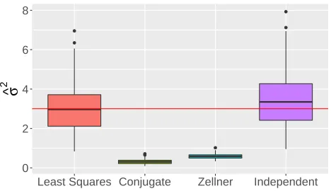
In Figure 1, we display a boxplot of the estimates ofσ2 _{for (i) Least Squares, (ii) Conjugate}

Bayesian ridge regression, (iii) Zellner’s prior:

β|σ2∼N(0, σ2τ2[XTX]−1), (2.19)

and (iv) Independent Bayesian ridge regression over 100 replications. Here, the estimates

from least squares and the independent ridge are reasonably distributed around the truth.

In sharp contrast, the estimates from the conjugate ridge and Zellner’s prior consistently

underestimate the error variance with medians of _bσ2 = 0.27 and 0.55, respectively. This

poor performance is a result of the bias induced by adding p “pseudo-observations” of σ2

as discussed in Section 2.3.1, which also occurs for the Zellner prior.

In the above simulation study, we considered the posterior mean of σ2 over many

repli-cations of the data. This allowed us to assess the variability of these point estimates in

a frequentist sense. For a Bayesian perspective, we can also consider the entire marginal

posterior distribution forσ2_{. For the conjugate prior formulation, this posterior is given by:}

σ2|Y∼IG

n

2,

YT[I−Hτ]Y

2

. (2.20)

The above distribution (2.20) is tightly concentrated about the posterior mode, given by

YT[I−Hτ]Y/(n+ 2), which suffers from the same underestimation phenomenon as the

posterior mean (2.16). Thus, consideration of the posterior distribution of σ2 will yield

● ●

● ●

●

● ●

0 2 4 6 8

Least Squares Conjugate Zellner Independent

σ

^

2

Figure 1: Estimatedσ_b2 _{for each procedure over 100 repetitions. The trueσ}2_{= 3 is the red}

horizontal line.

This phenomenon of underestimating σ2 can also be seen in EMVS (Roˇckov´a and George,

2014), which can be viewed as iterative Bayesian ridge regression with an adaptive penalty

term for each regression coefficient βj instead of the same τ2 above. EMVS also uses a

conjugate prior formulation in which β depends on σ2 a priori similarly to (2.10). As in

the above ridge regression example, with this prior EMVS yields good estimates forβ, but

severely underestimates σ2_{. This occurs in the Section 4 example of Roˇckov´a and George}

(2014) with n= 100 and p = 1000. There, conditionally on the modal estimate of β, the

associated modal estimate ofσ2_{is 0.0014, a severe underestimate of the true varianceσ}2 _{= 3.}

Fortunately, EMVS can be easily modified to use the independent prior specification, as

now has been done in the publicly available EMVS R package (Roˇckov´a and Moran, 2018).

It is interesting to note that the SSVS procedure of George and McCulloch (1993) used the

nonconjugate independence prior formulation in lieu of the conjugate prior formulation for

the continuous spike-and-slab setup.

A natural question to ask is: how does the poor estimate of the variance in the conjugate

case affect the estimated regression coefficients? Insight is obtained by comparing (2.15) to

the conditional posterior mean of β in the independent case, given by:

E[β|σ2,Y] =

XTX+σ

2

τ2I

−1

In (2.15), the Gaussian prior structure allows forσ2_{to be factorized out so that the estimate}

ofβdoes not depend on the variance. This lack of dependence on the variance is troubling,

however, as we want to select fewer variables when the error variance is large making the

signal-to-noise ratio low. This is in contrast to (2.21) where when σ2 is large relative to

τ2, the signal-to-noise ratio is low and so the posterior estimate for βwill be close to zero,

correctly reflecting the relative lack of information. This does not occur for the posterior

mean ofβ in the conjugate case.

Although the posterior mean of β in the conjugate prior formulation does not depend on

σ2_{, the posterior variance ofβdoes depend on the error variance. Specifically, the posterior}

variance of β is given by:

E[β|Y, σ2] =σ2[XTX+τ−2I]−1. (2.22)

Consequently, underestimation of σ2 will result in too narrow credible intervals forβ.

Fur-ther, underestimation of the error variance σ2 will also result in too narrow prediction

intervals for future responses.

2.3.3. What About a Prior Degrees of Freedom Adjustment?

At this point, one may wonder: if the problem seems to be the extraσp _{in the denominator,}

why not use the prior π(σ2_{) ∝ σ}p−4 _{instead of the right-Haar prior π(σ}2_{) ∝ σ}−2 _{that is}

commonly used? This “p-sigma” prior then results in the joint prior:

π(β|σ2)π(σ2)∝ 1

(σ2₎2exp

− 1

2σ2_τ2kβk

2

, (2.23)

which yields the implicit conditional prior onσ2_:

σ2|β∼IG

1,kβk

2

2τ2

For the simulation setup in Section 2.3.2, this alternative conjugate prior would in fact

remedy the variance estimates of the conjugate formulation (2.10). However, the p-sigma

prior can actually lead to overestimation of the error variance, as opposed to the

under-estimation observed in Section 2.3.1. Heuristically, the mean of the prior (2.24) is now of

order O(q), where q is the number of non-zeroβ. As many posterior concentration results

require q → ∞, albeit at a much slower rate thanp (see, for example, van der Pas et al.,

2016), this is particularly troublesome.

This overestimation can be further seen from the concentration of the prior captured in

Proposition 2 below. As we will discuss in Section 2.4, a similar phenomenon also occurs

for a penalized likelihood procedure that implicitly uses a p-sigma prior.

Proposition 2. Supposekβk₀ =qandminj,βj6=0β

2

j =K for some constantK∈R. Denote

the true variance as σ₀2. Then

P(σ2 ≥δσ₀2 |β)≥1−exp

− qK

2δσ2

0τ2

. (2.25)

Proof. We have:

P(σ2 ≥δσ₀2 |β) =

Z ∞

δσ2

0

kβk2

2τ2

1

u2 exp

−kβk

2

2τ2

1 u

du

≥1−exp

− qK

2δσ2

0τ2

.

Proposition 2 implies that we can choose arbitrary δ >1 such that asq → ∞, thep-sigma

prior places increasing mass on values of σ2 greater than δσ₀2. Another concern regarding

thep-sigma prior is more philosophical. As p gets larger, thep-sigma prior puts increasing

mass on larger and larger values ofσ2, which does not seem justifiable.

For these reasons, we prefer the independent prior forms for the regression coefficients and

error variance. We are also of the opinion that the simplicity of the independent prior is in

2.4. Connections with Penalized Likelihood Methods

Here we pause briefly to examine connections between Bayesian methods and developments

in estimating the error variance in the penalized regression literature. Such connections can

be drawn as penalized likelihood methods are implicitly Bayesian; the penalty functions

can be interpreted as priors on the regression coefficients so these procedures also in effect

yield MAP estimates.

One of the first papers to consider the unknown error variance case for the Lasso was St¨adler

et al. (2010), who suggested the following penalized loss function for introducing unknown

variance into the frequentist Lasso framework:

Lpen(β, σ2) =

kY−Xβk2

2σ2 +

λ

σkβk1+nlogσ. (2.26)

Optimizing this objective function is in fact equivalent to MAP estimation for the following

Bayesian model with the p-sigma prior discussed in Section 2.3.2:

Y∼N(Xβ, σ2I) (2.27)

π(β|σ2)∝ 1

σp

p

Y

j=1

e−λ|βj|/σ

π(σ2)∝σp.

Interestingly, Sun and Zhang (2010) proved that the resulting estimator for the error

vari-ance overestimates the noise level unless λkβ∗k1/σ∗ =o(1), where β∗ and σ∗ are the true

values of the regression coefficients and error variance, respectively. However, this condition

requires q, the true number of non-zero β, to be of the following order (details in Section

2.9.2 of the Appendix).

q =opn/logp. (2.28)

posterior contraction and result in consistent estimates for the error variance. Note also

the connection to Proposition 2: there, the prior mass on σ2 will concentrate on values

greater than the true variance unlesskβk2/τ2 =o(1).

To resolve this issue of overestimating the error variance, Sun and Zhang (2012) proposed

as an alternative the “scaled Lasso”, an algorithm which minimizes the following penalized

joint loss function via coordinate descent:

Lλ(β, σ) =

kY−Xβk2

2σ +

nσ

2 +λ

p

X

j=1

|βj|. (2.29)

This loss function is a penalized version of Huber’s concomitant loss function, and so may

be viewed as performing robust high-dimensional regression. It is also equivalent to the

“square-root Lasso” of Belloni et al. (2014). Minimization of the loss function (2.29) can

be viewed as MAP estimation for the Bayesian model (with a slight modification):

Y∼N(Xβ, σI) (2.30)

π(β)∝

p

Y

j=1 λ

2e

−λ|βj|

σ∼Gamma(n+ 1, n/2).

Note that to interpret the scaled Lasso as a Bayesian procedure, σ, rather than σ2_{, plays}

the role of the variance in (2.30). Sun and Zhang (2012) essentially then re-interpret σ

as the standard deviation again after optimization of (2.29). This re-interpretation can be

thought of as an “unbiasing” step for the error variance. It is a little worrisome, however,

that the implicit prior on the error variance is very informative: as n → ∞, this Gamma

prior concentrates around σ= 2.

Sun and Zhang (2012) proved that the scaled Lasso estimate _bσ(X,Y) is consistent for the

“oracle” estimator

σ∗= kY−Xβ

∗_k

√

where β∗ are the true regression coefficients, for the value of λ0 ∝

p

(2/n) logp. This

estimator (2.31) is called the oracle because it treats the true regression coefficients as if

they were known. The termkY−Xβ∗k2is then simply the sum of normal random variables,

of which we calculate the variance asPn

i=1ε2i/n.

2.5. Global-Local Shrinkage

In this section, we examine how the use of a conjugate prior affects the machinery of the

Gaussian global-local shrinkage paradigm. The general structure for this class of priors is

given by:

βj ∼N(0, τ2λ2_j), λ2_j ∼π(λ2_j), j= 1, . . . , p (2.32)

τ2 ∼π(τ2)

whereτ2 is the “global” variance andλ2_j is the “local” variance. Note that taking τ2 to be

the same as the error variance σ2 _{would result in a conjugate prior in this setting. This}

is exactly what was done in the original formulation of the Bayesian lasso by Park and

Casella (2008), which can be recast in the Gaussian global-local shrinkage framework as

follows (notation changed slightly for consistency):

Y|β, σ2∼Nn(Xβ, σ2In) (2.33)

βj|σ2, λ2j ∼N(0, σ2λ2j), π(λ2j) =

u2

2 e

−u2_λ2

j/2_{, j= 1, . . . , p}

π(σ2)∝σ−2.

In the conjugate formulation (2.33),σ2 plays the dual role of representing the error variance

as well as acting as the global shrinkage parameter. This is problematic in light of the

mechanics of global-local shrinkage priors. Specifically, Polson and Scott (2010) recommend

the following requirements for the global and local variances in (2.32): π(τ2_{) should have}

are negligible; and π(λ2

j) should have heavy tails so that it can be quite large, allowing for

a few large coefficients to “escape” the heavy shrinkage of the global variance.

This heuristic is formalized in much of the shrinkage estimation theory. For the normal

means problem where X = In and β ∈ Rn, van der Pas et al. (2016) prove that the

following conditions result in the posterior recovering nonzero means with the optimal rate:

(i) π(λ2_j) should be a uniformly regular varying function which does not depend on n; and

(ii)τ2 ₌ q

nlog(n/q), whereq is number of non-zeroβj.

The uniformly regular varying property in (i) intuitively preserves the “flatness” of the prior

even under transformations of the parameters, unlike traditional “non-informative” priors

(Bhadra et al., 2016). In preserving these heavy tails, such priors for λ2_j allow for a few

large coefficients to be estimated. The condition (ii) encourages τ2 to tend to zero which

would be a concerning property if it were also the error variance. These results suggest

we cannot identify the error variance with the global variance parameter on the regression

coefficients as in (2.33): it cannot simultaneously both shrink all the regression coefficients

and be a good estimate of the residual variance. Finally, we note that Hans (2009) also

considered the independent case for the Bayesian lasso in which the error variance is not

identified with the global variance.

An alternative conjugate formulation for Gaussian global-local shrinkage priors is to instead

include three variance terms in the prior forβj: the error variance,σ2, the global variance,

τ2, and the local variance,λ2_j. For example, Carvalho et al. (2010) give the conjugate form

of the horseshoe prior:

βj|σ2, τ2, λ2j ∼N(0, σ2τ2λ2j), λ2j ∼π(λ2j), j= 1, . . . , p (2.34)

τ2 ∼π(τ2),

π(σ2)∝σ−2.

separates the roles of the error variance and global variance. However, this prior structure

can still be problematic for error variance estimation.

Consider the conditional posterior mean ofσ2 for the model (2.34):

E[σ2|Y,β, τ2, λ2j] =

kY−Xβk2+Pp

j=1βj2/λ2jτ2

n+p−2 . (2.35)

Proposition 3 highlights that, given the true regression coefficients, the conditional posterior

mean ofσ2 underestimates the oracle variance (2.31) whenβ is sparse.

Proposition 3. Consider the global-local prior formulation given in (2.34). Denote the

true vector of regression coefficients by β∗ where kβ∗k₀ = q. Suppose maxjβj∗2 =M1 for

some constantM1 ∈R. Denote the oracle estimator forσgiven in (2.31)byσ∗ and suppose

σ∗ _{=O(1). Suppose also that for j ∈ {1, . . . , p} with β}

j 6= 0, we have τ2λ2j > M2 for some

M2 ∈R. Then

E[σ2|Y,β∗, τ2, λ2j]≤

nσ∗2

n+p−2 +

q

n+p−2

M1

M2

. (2.36)

In particular, as p/n→ ∞ and q/p→0, we have

E[σ2|Y,β∗, τ2, λ2j] =o(1). (2.37)

Given the mechanics of global-local shrinkage priors, the assumption in Proposition 3 that

the termτ2λ2_j is bounded from below for non-zeroβj is not unreasonable. This is because for

largeβj, the local varianceλ2j must be large enough to counter the extreme shrinkage effect

ofτ2. Indeed, the prior forλ2_j must have “heavy enough” tails to enable this phenomenon.

We should note that Proposition 3 illustrates the poor performance of the posterior mean

(2.35) given the true regression coefficients β∗, whereas the horseshoe procedure does not

actually threshold the negligibleβjto zero in the posterior mean ofβ. For these smallβj, the

termτ2_λ2

However, it is still troubling to use an estimator for the error variance that does not behave

as the oracle estimator when the true regression coefficients are known. This is in contrast

to the independent prior formulation where the conditional posterior mean ofσ2 is simply:

E[σ2|Y,β] =

kY−Xβk2

n−2 . (2.38)

Note also that the problem of underestimation of σ2 is exacerbated for modal estimation

under the prior (2.34). This is because modal estimators often threshold small coefficients

to zero and so the term Pp

j=1βj2/λ2jτ2 becomes negligible as in Proposition 3. As MAP

estimation using global-local shrinkage priors is becoming more common (see, for example,

Bhadra et al., 2017), we caution against the use of these conjugate prior forms.

A different argument for using conjugate priors with the horseshoe is given by Piironen and

Vehtari (2017). They advocate for the model (2.34), arguing that it leads to a prior on the

effective number of non-zero coefficients which does not depend onσ2 andn. However, this

quantity is derived from the posterior ofβand so does not take into account the uncertainty

inherent in the variable selection process. As a thought experiment: suppose that we know

the error variance, σ2, and number of observations, n. If the error variance is too large

and the number of observations are too few, we would not expect to be able to say much

about β at all, and this intuition should be reflected in the effective number of non-zero

coefficients. This point is similar to our discussion at the end of Section 2.3.2 regarding

estimation of β.

As before, we recommend independent priors on both the error variance and regression

coefficients to both prevent distortion of the global-local shrinkage mechanism and to obtain

2.6. Spike-and-Slab Lasso with Unknown Variance

2.6.1. Spike-and-Slab Lasso

We now turn to the Spike-and-Slab Lasso (SSL, Roˇckov´a and George, 2018) and consider

how to incorporate the unknown variance case. The SSL places a mixture prior on the

regression coefficients β, where each βj is assumed a priori to be drawn from either a

Laplacian “spike” concentrated around zero (and hence be considered negligible), or a diffuse

Laplacian “slab” (and hence may be large). Thus the hierarchical prior overβand the latent

indicator variablesγ= (γ1, . . . , γp) is given by

π(β|γ)∼

p

Y

j=1

[γjψ1(βj) + (1−γj)ψ0(βj)], (2.39)

π(γ|θ) =

p

Y

j=1

θγj_(1−θ)1−γj _{and θ∼Beta(a, b),}

where ψ1(β) = λ1

2 e

−|β|λ1 _{is the slab distribution and ψ0(β) =} λ0

2 e

−|β|λ0 _{is the spike (λ1}

λ0), and we have used the common exchangeable beta-binomial prior for the latent

indica-tors.

Roˇckov´a and George (2018) recast this hierarchical model into a penalized likelihood

frame-work, allowing for the use of existing efficient algorithms for modal estimation while

retain-ing the adaptivity inherent in the Bayesian formulation. The regression coefficients β are

then estimated by

b

β= arg max

β∈_Rp

−1

2kY−Xβk

2_+pen(β)

(2.40)

where

pen(β) = log

π(β)

π(0p)

, π(β) =

Z 1

0 p

Y

j=1

Roˇckov´a and George (2018) note a number of advantages in using a mixture of Laplace

densities in (2.39), instead of the usual mixture of Gaussians as has been standard in the

Bayesian variable selection literature. First, the Laplacian spike serves to automatically

threshold modal estimates of βj to zero when βj is small, much like the Lasso. However,

unlike the Lasso, the slab distribution in the prior serves to stabilize the larger coefficients

so they are not downward biased. Additionally, the heavier Laplacian tails of the slab

distribution yields optimal posterior concentration rates (Roˇckov´a, 2018).

Although the use of the spike-and-slab prior is typically associated with “two-group” Bayesian

variable selection methods, the Spike-and-Slab Lasso can also be interpreted as a

“one-group” global-local shrinkage method as the spike density is continuous. As such, the use

of a conjugate prior for the error variance here will result in underestimation, similarly to

the results for global-local shrinkage priors in Section 2.5. This is especially the case as

the SSL procedure finds the modes of the posterior, automatically thresholding negligible

regression coefficients to zero. In the next section, we provide further details on why this

underestimation phenomenon occurs for the SSL with a conjugate prior formulation.

Af-terwards, we introduce the SSL with unknown variance which avoids this underestimation

problem by instead utilizing an independent prior framework.

2.6.2. The Failure of a Conjugate Prior

This conjugate prior formulation for the Spike-and-Slab Lasso is given by:

π(β|γ, σ2)∼

p

Y

j=1

γj

λ1

2σe

−|βj|λ1/σ_{+ (1−γ}

j)

λ0

2σe

−|βj|λ0/σ

(2.42)

γ|θ∼

p

Y

j=1

θγj_(1−θ)1−γj_{, θ∼Beta(a, b) (2.43)}

p(σ2)∝σ−2. (2.44)

can be found in Section 2.9.3 of the Appendix. At the (k+ 1)th iteration, the EM update

for the error variance is:

σ(k+1)= Q+

q

Q2_{+ 4(kY−Xβ}(k)_k2_{)(n+p+ 2)}

2(n+p+ 2) (2.45)

with

Q=

p

X

i=1

|β_j(k)|λ∗(β_j(k)/σ(k);θ(k)), (2.46)

λ∗(β;θ) =λ1p∗(β;θ) +λ0(1−p∗(β;θ)), (2.47)

p∗(β;θ) =

1 +λ0

λ1

1−θ

θ

exp{−|β|(λ0−λ1)}

−1

, (2.48)

whereβ(k), σ(k), θ(k) are the parameter values after the kth iteration.

Let us take a closer look at the update (2.45). Following the line of reasoning in Sun and

Zhang (2010), an expert with oracle knowledge of the true regression coefficientsβ∗ would

estimate the noise level by the oracle estimator:

σ∗2= kY−Xβ

∗_k

n . (2.49)

However, the maximuma posteriori estimate ofσ at the true values ofβ∗,γ∗ _{is given by}

b

σM AP =τ+

s

τ2₊ (σ∗)2

1 +p/n+ 2/n (2.50)

where τ = λ1kβ∗k1/[2(n+p+ 2)]. Here we see that if n → ∞ with p fixed, we have

b

σM AP → σ∗. If, however, we have p/n → ∞ and q/p → 0, where the underlying sparsity

is q = kβ∗k₀, we have bσM AP → 0. Thus, similarly to our previous examples in Sections

2.3 and 2.5, we will severely underestimate the error variance. As in these examples, the

2.6.3. Spike-and-Slab Lasso with Unknown Variance

We now introduce the Spike-and-Slab Lasso with unknown variance, which considers the

regression coefficients and error variance to bea prioriindependent. The hierarchical model

is

π(β|γ)∼

p

Y

j=1

[γjψ1(βj) + (1−γj)ψ0(βj)] (2.51)

γ|θ∼

p

Y

j=1

θγj_(1−θ)1−γj_{, θ∼Beta(a, b) (2.52)}

π(σ2)∝σ−2. (2.53)

The log posterior, up to an additive constant, is given by

L(β, σ2) =− 1

2σ2kY−Xβk

2_{−(n+ 2) logσ+}

p

X

j=1

pen(βj|θj) (2.54)

where, for j= 1, . . . , p,

pen(βj|θj) =−λ1|βj|+ log[p∗(0;θj)/p∗(βj;θj)], (2.55)

with p∗(β;θ) = θψ1(β)

θψ1(β) + (1−θ)ψ0(β) and θj =E[θ|β\j]. (2.56)

For large p, Roˇckov´a and George (2018) note that the conditional expectation E[θ|β\j] is

very similar to E[θ|β] and so for practical purposes we treat them as equal and denote

θβ =E[θ|β].

To find the modes of (2.54), we pursue a similar coordinate ascent strategy to Roˇckov´a

and George (2018), cycling through updates for each βj and σ2 while updating the

however, Roˇckov´a and George (2018) note that it can be approximated by

θβ ≈

a+kβk0

a+b+p. (2.57)

We now outline the estimation strategy for β. As noted in Lemma 3.1 of Roˇckov´a and

George (2018), there is a simple expression for the derivative of the SSL penalty:

∂pen(βj|θβ)

∂|βj| ≡ −λ

∗_(β

j;θβ) (2.58)

where

λ∗(βj;θβ) =λ1p∗(βj;θβ) +λ0[1−p∗(βj;θβ)]. (2.59)

Using the above expression, the Karush-Kuhn-Tucker (KKT) conditions yield the following

necessary condition for the global mode β:b

b

βj =

1 n

h

|zj| −σ2λ∗(βb_j;θ_β) i

+sign(zj), j= 1, . . . , p (2.60)

wherezj =XTj(Y−

Pp

k6=jβb_k·X_k) and we assume that the design matrixXhas been centered

and standardized to have norm √n. The condition (2.60) is very close to the familiar

soft-thresholding operator for the Lasso, except that the penalty term λ∗(βj;θ) differs for

each coordinate. Similarly to other non-convex methods, this enables selective shrinkage

of the coefficients, mitigating the bias issues associated with the Lasso. As a non-convex

method, however, (2.60) is not a sufficient condition for the global mode. This is particularly

problematic when the posterior landscape is highly multimodal, a consequence of p n

and large λ0. To eliminate many of these suboptimal local modes from consideration,

Roˇckov´a and George (2018) develop a more refined characterization of the global mode.

This characterization follows the arguments of Zhang and Zhang (2012) and can easily be

Proposition 4. The global mode βb satisfies

b

βj =

   

  

0 when |zj| ≤∆

1

n[|zj| −σ2λ∗(βjb;θβ)]+sign(zj) when |zj|>∆

(2.61)

where

∆≡inf

t>0[nt/2−σ

2_pen(t|θ

β)/t]. (2.62)

Unfortunately, computing (2.62) can be difficult. Instead, we seek an approximation to the

threshold ∆. A useful upper bound is ∆≤σ2λ∗(0;θβ) (Zhang and Zhang, 2012). However,

when λ0 gets large, this bound is too loose and can be improved. The improved bounds

are given in Proposition 5, the analogue of Proposition 3.2 of Roˇckov´a and George (2018)

for the unknown variance case. Before stating the result, the following function is useful to

simplify exposition:

g(x;θ) = [λ∗(x;θ)−λ1]2+

2n

σ2 log[p

∗_{(x;θ)]. (2.63)}

Proposition 5. When σ(λ0−λ1)>2√nand g(0;θβ)>0 the threshold∆ is bounded by

∆L<∆<∆U,

where

∆L=

q

2nσ2_log[1/p∗_(0;θ

β)]−σ4dj+σ2λ1, (2.64)

∆U =q2nσ2_log[1/p∗_(0;θ

β)] +σ2λ1 (2.65)

and

0< dj <

2n

σ2 −

n

σ2_(λ

0−λ1)

− √

2n σ

!2

.