Modeling And Computational Fluid Flow Analysis
Of Cryogenic Turboexpander
1U.Bhagyaraju, 2P.Tagore Kumar 1PG M.Tech Student, 2Assistant Professor 1QIS College of Engineering & Technology Ongole,
2QIS College of Engineering & Technology Ongole
_____________________________________________________________________________________________________
Abstract - Cryogenic turboexpander is the most critical component of cryogenic plant to achieve low temperature
refrigeration. A cryogenic turboexpander has many components like expansion turbine, compressor, heat exchanger, instrumentations etc. Expansion turbine is the component where temperature of gases decreases due to expansion and produce the coldest level of refrigeration in the plant. In this paper deals with the computational fluid flow analysis of high-speed expansion turbine. This involves with the three-dimensional analysis of flow through a radial expansion turbine using nitrogen as flowing fluid. This analysis is done using CFD packages, bladegen, turbogrid and CFX. Bladegen is used to create the model of turbine using available data of hub, shroud and blade profile. Turbogrid is used to mesh the model. CFX-Pre is used to define and specify the simulation settings and physical parameters required to describe the flow through turboexpander at inlet and outlet. CFX-Post is used for examining and analyzing results. Using these results variation of different thermodynamic properties inside the turbine can be seen. Various graphs are potted indicating the variation of velocity, pressure, temperature, entropy and Mach number along streamline and span wise to analyze the flow through cryogenic turbine.
keywords - Radial turbine, Bladegen, Turbogrid, CFX
_____________________________________________________________________________________________________
1.INTRODUCTION
Turboexpander are used in all areas of the gas and oil industries to produce cryogenic refrigeration. A turboexpander, on other hand, is a pressure let-down device that produces cryogenic temperature while simultaneously recovering energy from a plant stream in form of shaft power that can be used to drive other machinery such as compressor. Collins, S. C et.al [1] studied the concept that an expansion turbine might be used in a cycle for the liquefaction of gases and the use of a turbine instead of a piston expander for the liquefaction of air. Sixsmith, H. et.al [2], a report was published on the first successful commercial application for cryogenic expansion turbine at the Linde works in Germany. Swearingen, J. S. et.al [3] description of a low temperature turboexpander w a s attaining 83% efficiency. It had an 8 cm Monel wheel with straight blades and operated at 40,000 rpm a turboexpander was developed which operated without trouble for periods aggregating 2,500 hrs and attained an efficiency of more than 80%.Clarke, M. E. et.al[4] experimentally investigated on the small gas bearing turboexpander commenced in the early fifties by Sixsmith at Reading University on a machine for a small air liquefaction plant. Beasley, S. A. et.al [5] d ev e l op ed a r a d i a l i n w a r d f l o w t u r b i n e for a nitrogen production plant. Swearingen,
J. S. et.al [6] developed during 1958 to 1961 Stratos Division of Fairchild Aircraft built blower loaded turboexpanders,
mostly for air separation service Voth et. al [7] developed a high- s p e e d turbine expander as a part of a cold moderator refrigerator for the Argonne National Laboratory (ANL). The first commercial turbine using helium was operated in 1964 in a refrigerator that produced 73 W at 3 K for the Rutherford helium bubble chamber.
Colyer, D. B [8] and Gessner, R. L et.al [9] A high speed turboalternator was developed by G. E. Co., New York
in 1968, which ran on a practical gas bearing system capable of operating at cryogenic temperature with low loss. Sixsmith,
H. et.al [10] developed a turbine with shaft diameter of 8 mm. This turbine operated at a speed of 600,000 rpm at 30K
inlet temperature. Schmid, C. et.al [11] developed a turboexpander f or cryogenic plants with self-acting gas bearings.
Reuter K.et.al [12] development program together with a magnetic bearing manufacturer to develop a cryogenic
turboexpander incorporating active magnetic bearing in both radial and axial direction. Reuter K. et.al [13] developed a micro turboexpander for a small helium refrigerator based on Claude cycle. This turboexpander consisted of a radial inward flow reaction turbine and a centrifugal brake fan on the lower and upper ends of a shaft supported by self-acting gas bearings. The turbine wheel diameter was 6mm and the shaft diameter was 4 mm. The rotational speeds of the 1st and 2nd stage turboexpander were 816,000 and 519,000 rpm respectively.
Based on the exhaustive literature for the development of computational fluid flow analysis of turboexpander system this paper has been initiated. The objectives include: (i) building computational fluid dynamic knowledge base on cryogenic turboexpanders (ii) construction of a computational fluid flow model and study of its performance.
2. COMPUTATIONAL FLUID FLOW ANALYSIS
and specify the simulation settings and physical parameters required to describe the flow through turboexpander at inlet and outlet. CFX-Post is used for examining and analyzing results.
2.1. Designing of Turboexpander in Bladegen
ANSYS BladeGen is a geometry creation tool that is specialized for turbomachinery blades. Bladegen designing of model is done by using available hub, shroud and blade profile coordinates. The hub and the tip streamlines are available in the previous chapter. A surface is created by joining the hub and tip streamlines with a set of tie lines. Blade Editor will loft the blade surfaces in the streamwise direction through curves that run from hub to shroud. The surface so generated is considered as the mean surface within a blade. Non-Uniform Rational B Splines are used to develop the solid surface. The suction and pressure surfaces of two adjacent channels are computed by translating the mean surface in the positive and negative theta direction through half the blade thickness.
After making all the surfaces when blade merge topology property is used, then blade faces will be merged where they are tangent to one another. Create fluid zone property is selected, to create a stage fluid zone body for the flow passage, and an enclosure feature to subtract the blade body. This resulting enclosure can be used for a CFD analysis of the blade passage. Create all blades this property is used to create all the blades using the number of blades specified in the Bladegen model as ass shown in Fig 2.1
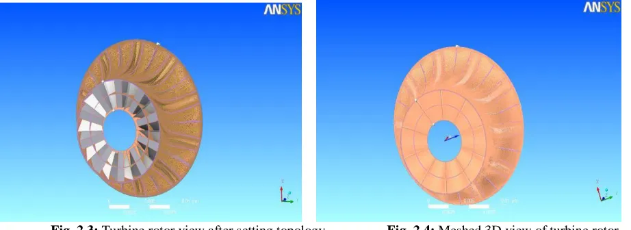
Fig. 2.1: Wireframe model of turbine generated in bladegen Fig. 2.2: Turbine rotor view after importing from Bladegen
2.2. Meshing of Model
Meshing of model is done in turbogrid. It creates high quality hexahedral meshes that are tuned to the demands of fluid dynamic analysis in turbine rotor. Turbine rotor geometry information is imported from bladegen. Turbogrid uses this bladegen file to set the axis of rotation, the number of blades, and a length unit that characterizes the scale of the machine. Machine data gives the basic information about the geometry. Here units specified for base units represent the scale of the geometry being meshed, these units are not used for importing geometric data nor do they govern the units written to a mesh file, they are used for the internal representation of the geometry to minimize computer round-off errors. To complete the geometry a small gap of 1 mm is created between the blade and the shroud as shown in Fig.2.2.
Next step is to create the topology that guides the mesh. Topology definition, placement to traditional with control points provides access to the legacy topology methods. Here H/J/C/LGrid method is used to create mesh. The H/J/C/L-Grid method causes ANSYS Turbogrid to choose an H-Grid, J-Grid, C-Grid, L-Grid, or a combination of these, based on heuristics. In this case, the H/J/C/L-Grid method causes ANSYS Turbogrid to choose an H-Grid topology for the upstream end of the passage, and an H-Grid topology for the downstream end. Include O-Grid with 0.5 width factor is selected to add an O-Grid (thickness equal to half the average blade thickness) around the blade to increase mesh orthogonality in that region as shown in Fig.2.3.
layers, especially the hub and shroud tip layers. After correcting mash quality on layers, we generate the mesh with 228640 nodes and 206368 elements as shown in Fig.2.4.
2.3. Physics definition of Meshed Model in CFX-Pre:
CFX-Pre is known as physics-definition pre-processor for ANSYS CFX. In CFX, turbo mode is used to define physic of meshed turbine rotor. Under basic setting in turbo mode, we set the machine type as radial turbine and rotation axis to z. In component definition we set component type rotating and set rotation value 218780 rev/min. Turbo mode will automatically select a list of regions that correspond to certain boundary types. This information should be reviewed in the Region Information section to ensure that all is correct. This information is used to set up boundary conditions and interfaces. In wall configuration option we set tip clearance at shroud. Physics definition tab is used to set fluid type, analysis type, model data, inflow and outflow boundary templates and solver parameters. Physics definition used for turbine rotor is given in the table below.
Table 2.1: Physics definition for turbine rotor
Tab Setting Values
Physics Definition
Fluid Nitrogen
Analysis Type Steady state
Modal Data
Reference pressure 0 (Pa) Heat Transfer Total Energy
Turbulence k-Epsilon
Inflow/Outflow Boundary Templates Mass Outlet Flow Inlet P-Static
Inflow
T-Total 99.65k
Mass Flow Per Component
Mass Flow Rate 0.002326 kg/sec Flow Direction Normal to Boundary
Outflow P-Static 1.29 bar
Solver Parameters
Advection Scheme High Resolution Convergence control Physical Timescale Physical Timescale 0.000004 s
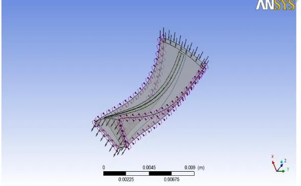
After setting physics definition CFX-Pre will try to create appropriate interfaces and boundary conditions using the region names presented previously in the region information as shown in Fig.2.5
Fig.2.5: Flow direction at inlet and outlet
3. RESULTS AND DISCUSSION
The computational fluid flow analysis is done in CFD post after completion of CFX simulation. A tabulated result can be seen in generated report. This report gives the variation of different properties from inlet to outlet and hub to shroud, by graphs and counters. Variations of thermodynamic properties, at different locations of turbine rotor are as following.
Table 3.1: Variations of thermodynamic properties
Quantity Inlet LE Cut TE Cut Outlet TE/LE Units
Density 8.5944 8.4588 4.7636 4.5933 0.5631
[kg m-3]
Pstatic 244299 241899 125866 127695 0.5203 [Pa]
Ptotal 300332 295012 173430 166980 0.5879 [Pa]
Ptotal (rot) 300241 292385 194824 187423 0.6663 [Pa]
Ttotal 99.6526 98.5519 96.7926 96.8437 0.9684 [K]
Ttotal (rot) 99.6435 99.6405 99.6466 99.7047 1.0001 [K]
Entropy 5377.19 5385.71 5512.42 5524.16 1.0235
[J kg-1 K-1]
Mach (abs) 0.784 0.7449 0.6667 0.6011 0.8949
Mach (rel) 1.2649 1.1969 0.9175 0.8663 0.7665
U 186.972 182.671 94.5048 92.5352 0.5173
[m s-1]
From tabulated results we can see that inside the turbine, pressure, temperature, density, velocity and Mach number are decreasing from inlet to outlet while entropy is increasing a little bit from inlet to outlet.
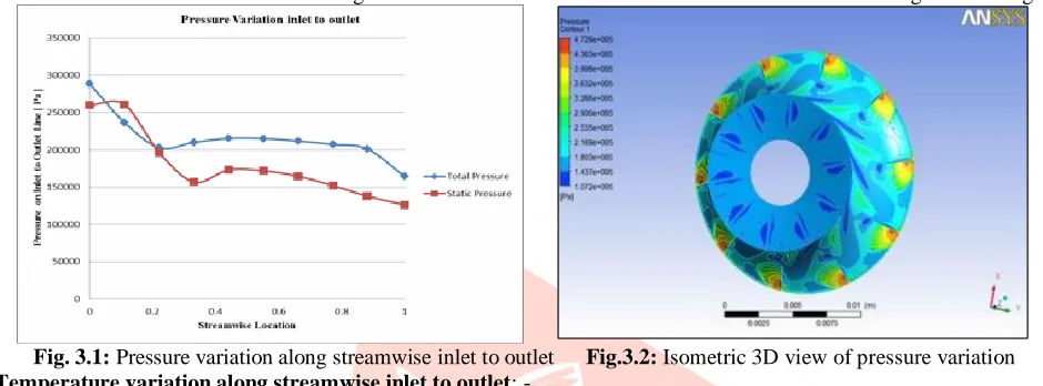
3.1 Pressure variation along streamwise inlet to outlet:
Static and total pressure variation can be seen from the graph below. Total pressure at inlet and static pressure at outlet is nearly equal to the pressure obtained by S.K.Ghosh [14] experimentally. Total pressure varies from 3bar to 1.6 bar while static pressure varies from 2.4 bar to 1.27 bar along streamline from inlet to outlet of turbine rotor as shown in Fig. 3.1 and Fig. 3.2
Fig. 3.1: Pressure variation along streamwise inlet to outlet Fig.3.2: Isometric 3D view of pressure variation 3.2 Temperature variation along streamwise inlet to outlet: -
Static and total temperature variation can be seen from the graph below. Total temperature at inlet and static temperature at outlet is nearly equal to the temperature obtained by S.K. Ghosh [14] experimentally. Total temperature varies from 99.6K to 96.7K, while static temperature varies from 95.82K to 88.67K along streamline from inlet to outlet of turbine rotor as shown in Fig. 3.3 and Fig. 3.4.
.
Fig.3.3: Temperature variation along streamwise inlet to outlet Fig.3.4: Isometric 3D view of temperature variation 3.3 Velocity variation along streamwise inlet to outlet:
Velocity variation can be seen from the graph below. Velocity is decreasing inside the turbine from inlet to outlet, 186.90 m/s to 130.146m/s respectively as shown in Fig. 3.5
Fig.3.5: Velocity variation along streamwise inlet to outlet Fig.3.6: Variation of Mach number along streamwise 3.4 Variation of Mach number along streamwise:
Absolute and relative Mach number variation can be seen from the graph below. Absolute Mach number varies from 0.7 to 0.89, while relative Mach number varies from 1.2 to 0.45 along streamline from inlet to outlet, inside the turbine rotor. as shown in Fig. 3.6.
3.5 Variation of density along streamwise inlet to outlet:
Density variation can be seen from the graph below. Density is decreasing inside the turbine from inlet to outlet, 8.59 kg/m3 to 4.59 kg/m3 respectively as shown in Fig. 3.7.
Fig.3.7: Variation of density along streamwise inlet to outlet Fig.3.8: Variation of Static Entropy along streamwise
3.6 Variation of Static Entropy along streamwise:
Static Entropy variation can be seen from the graph below. Static Entropy varies from 5377 J 1 K^-1 to 5524 J kg^-1 K^-kg^-1 along streamline from inlet to outlet, inside the turbine rotor, which shows that expansion process is not isentropic. A small increment in entropy can be seen from inlet to outlet, inside the turbine as shown in Fig. 3.8..
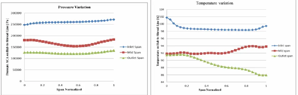
3.7 Pressure variation along spanwise hub to shroud:
Pressure variation at different span, hub to shroud can be seen from graph below. At inlet span, hub to shroud variation of pressure is around 2.48 bar to 2.67 bar, while at mid and outlet span pressure is varying around 1.7 bar to 1.8 bar and 1.26 bar to1.27 bar respectively as shown in Fig. 3.9.
.
Fig. 3.9: Pressure variation along spanwise hub to shroud Fig.3.10: Temperature variation along spanwise hub to shroud
3.8 Temperature variation along spanwise hub to shroud:
K and 91 K to86 K respectively as shown in Fig. 3.10.
3.9 Velocity variation along spanwise hub to shroud:
Velocity variation at different span, hub to shroud can be seen from graph below. At inlet span, hub to shroud variation of velocity is around 186 m/s to 188 m/s, while at mid and outlet span velocity is varying around 160 m/s to 130 m/s and 90 m/s to100 m/s respectively as shown in Fig. 3.11.
Fig.3.11: Velocity variation along spanwise hub to shroua Observation:
The gas flows radially inward, is accelerated through inlet guide vanes, and turned. The swirling, high velocity gas enters the expander impeller with relatively low incidence, because the blade tip velocity at the impeller outside diameter approximately matches the gas velocity. Work is extracted from the gas by removing this momentum: as the gas moves inward, it is forced to slow down because the blade rotational velocity decreases with the decreasing radius. The blades also turn the gas to reduce the gas velocity even further. As a result, the gas exits the impeller with low tangential velocity relative to the outside world. In this way, the angular momentum o f t h e g a s is efficiently r e m o v e d . Dew to this reason, different thermodynamic properties decrease from inlet to outlet.
3.10 Blade to blade plots for different spans: Contour of velocity vector at different Spans:
Fig.3.14: Velocity Vectors at 80% Span Observation:-
Above figures are showing the variation of velocity vectors at 20%, 50% and 80% spans from hub to shroud. Here we can see that velocity of fluid is decreasing from inlet to outlet and variation in velocity vectors are more complicate from hub to shroud. At 20% and 50% spans there is less space to move velocity vectors; while at 80% span (near to shroud) variation is more because of gap between blade tip and shroud.
3.11 Meridional Plots:
Contour of Mass Averaged Pressure on Meridional Surface
Fig.3.15: Mass Averaged Pressure on Meridional Surface Fig.3.16: Mass Averaged Relative Mach number on Meridional Surface
Contour of Mass Averaged Relative Mach number on Meridional Surface:- 3.12 Streamline Plot: -
Velocity Streamlines at Blade Trailing Edge: -
Fig.3.17: Velocity Streamlines at Blade Trailing Edge Observation
4. CONCLUSIONS AND FUTURE WORK 4.1. Conclusions
This work is a modest attempt at flow analyzing inside a cryogenic turboexpander through computational fluid dynamic. A prototype expander has been designed, meshed and simulated using this recipe. The design procedure covers the designing of hub, shroud and blade
profile of turboexpander in Bladegen. A CFX model has been developed for flow analysis inside the turbine rotor. The modeling of the various parts of the turbine is done in Bladegen and the computational fluid flow analysis is done using CFX. After validation of output results with experimental results, various graphs and contours indicating the variations of temperature, pressure, velocity, Mach number and entropy inside the turbine along the streamline and spanwise are drawn.
4.2. Future work
Future work in this direction will be aimed at computational fluid flow analysis of the
remaining parts of turboexpander like nozzle, diffuser, etc. It is expected that a complete model of turboexpander can be computationally analyzed by using proper designing and simulation tools. In this regard, work is planned on the application of CFX tool in mixing plane selection. Once it will be done then computational simulation of different types of turboexpander can be analyzed.
REFERNCES
[1] Collins, S.C. and Cannaday, R.L. Expansion Machines for Low Temperature Processes Oxford University Press (1958).
[2] Sixsmith, H. Miniature cryogenic expansion turbines - a review Advances in Cryogenic Engineering (1984), V29, 511-523.
[3] Swearingen, J. S. Turbo-expanders Trans AIChE (1947), 43 (2), 85-90
[4] Clarke, M. E. A decade of involvement with small gas lubricated turbine & Advances in Cryogenic Engineering (1974), V19, 200-208
[5] Beasley, S. A. and Halford, P. Development of a High Purity Nitrogen Plant using Expansion Turbine with Gas Bearing Advances in Cryogenic Engineering (1965),
V10B, 27-39
[6] Swearingen, J. S. Engineers' guide to turboexpanders Roto Flow Corp, USA, (1970), Gulf Publishing Company [7] Voth, R. O., Norton, M. T. and Wilson, W. A. A cold modulator refrigerator incorporating a high speed turbine
expander Advances in Cryogenic Engineering (1966), V11, 127-138
[8] Colyer, D. B. Miniature cryogenic refrigerator alternators Advances in Cryogenic Engineering (1968), V13, 405-415
[9] Colyer, D. B. and Gessner, R. L. Miniature cryogenic refrigerator Turbomachinery Advances in Cryogenic Engineering (1968), V13, 484-493
[10] Sixsmith, H. Miniature expansion turbines, C A Bailey (Ed), Advanced Cryogenics Plenum Press (1971), 225-243
[11] Schmid, C. Gas bearing turboexpanders for cryogenic plant 6th International Gas Bearing Symposium University of Southampton England (March 1974) Paper 131 B1: 1-8
[12] Reuter K. and Keenan B. A. Cryogenic turboexpanders with magnetic bearings AICHE Symposium Series, Cryogenic Processes and Machinery 89 (294), 35-45
[13] Izumi, H., Harada, S. and Matsubara, K. Development of small size Claude cycle helium refrigerator with micro turbo-expander Advances in Cryogenic Engineering (1986), V31, 811 818