98
Comparison On Matching Methods Used In Pose
Tracking For 3D Shape Representation
Khin Kyu Kyu Win, Yu Yu Lwin
Abstract: In this work, three different algorithms such as Brute Force, Delaunay Triangulation and k-d Tree, are analyzed on matching comparison for 3D shape representation. It is intended for developing the pose tracking of moving objects in video surveillance. To determine 3D pose of moving objects, some tracking system may require full 3D pose estimation of arbitrarily shaped objects in real time. In order to perform 3D pose estimation in real time, each step in the tracking algorithm must be computationally efficient. This paper presents method comparison for the computationally efficient registration of 3D shapes including free-form surfaces. Matching of free-form surfaces are carried out by using geometric point matching algorithm (ICP). Several aspects of the ICP algorithm are investigated and analyzed by using specified surface setup. The surface setup processed in this system is represented by simple geometric primitive dealing with objects of free-from shape. Considered representations are a cloud of points.
Index Terms: ICPalgorithm, matching technique, pose tracking, 3D shape representation, point cloud model
————————————————————
1
I
NTRODUCTIOND to the complexity of mutual relationship, simultaneous shape acquisition and pose estimation is necessary in interacting computer vision with the environment. The interactions include the applications of robotic, visual surveillance and recognizing human movement. The task of shape representation is to establish point-to-point correspondences between two images. To estimate the geometric transformation between the reference image and the 3D object, shape matching is used. Basic shape matching algorithm is the iterative closet points (ICP) algorithm in [1] that uses explicit representations like points and curves. ICP is a low level geometric matching algorithm and creates closest point correspondences between two sets of point data and model at each iteration. It minimizes the average distance between both sets by finding an optimal rigid transformation. The main difficulty of ICP algorithm is the requirements of heavy computations. Its complexity depends on the number of points of data sets. Matching detailed high resolution shapes takes too much time. To reduce ICP computation time, there can have the solutions to speed up the algorithm in different ways such as reducing number of iterations, reducing the number of data pints and accelerating the closet point search. In this paper, ICP algorithm is analysed by using three different closet point searches; Brute Force Search, Delaunay Triangulation and k-d Tree Search. For performance analysis, comparisons of these methods are simulated with changing number of data points and different shape representations. Their computation time, number of iterations and rms error are analysed for the optimized method for developing pose tracking of moving objects.
2
R
ELATEDW
ORKGenerally, 3D object modelling requires assembling several complementary views into a single representation. There are geometric representations such as points, lines and surfaces.
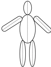
Geometric models describe the exact 3D shape of an object. For example, a person might be modelled as a generalized cylinder shown in Fig. 1. Extracting a point cloud of a real object from 3D surface measurement is a common task in reconstruction. An automatic method of point clouds merging for complete surface reconstruction is presented in [2].
Fig. 1 Rough Generalized Cylinder Model of a Person
The techniques ICP in based on the intrinsic properties of measured surfaces, or geometric matching is common approach for shape registration. Fast ICP for shape registration in [3] present the tree search method. It permits to reduce ICP complexity. Else rigid-body transformations in 3D relate different positions of a rigid object, or different 3D views of an object. The illustration in [4] shows experimentally on two applications, 3D object tracking and image registration with Iterative Closest Point.The performance improvement of ICP in [5] is tested using grid like structure to implement point-to-point matching. The data point-to-point in each cloud is approximately 6000. In [6], estimation of covariance is presented on ICP in 3D with point-to-point error metric.
3
M
ETHODOLOGYThe Iterative Closet Point (ICP) algorithm is briefly overviewed for aligning point clouds. In this paper, the point-to-point algorithm is considered among different variations of ICP.
3.1 Iterative Closet Point Algorithm
Several steps of point correspondence in the ICP algorithm in [1] iteratively perform matching, error minimization and transformation. The transformation to the data points require to bring the best alignment with the model points. The model point set will be denoted as:
__________________________
Khin Kyu Kyu Win is currently pursuing PhD degree program in electroic engineering in Yangon Technological University, Myanmar, PH-095401090. E-mail: [email protected]
Yu Yu Lwin is currently Head of Department in electroic engineering in Yangon Technological University, Myanmar, PH-951642404. E-mail:
99 Q = {q1, q2, q3,……., qN}
and the data point set can be denoted as:
P = {p1, p2, p3,……., pN}
Error metric is defined as the sum of squared errors. These errors are the squared distances from points in one cloud to their nearest neighbours after applying transformation. According to the task, transformations can be rigid or non-rigid. In 3D space, a transformation has three rotations and three translations. The objective function using point-to-point minimization can be expressed as:
∑‖ ‖
Where R is the rotation matrix and T is translation vector. The concept of standard ICP algorithm include two steps: computing correspondences and computing transformation to be minimized distance between corresponding points. The algorithm can be listed below.
Input: two pint clouds; Q = {qi}, P = {pi}
Initial transformation; R and T
Output : correct transformation to aligns Q and P
Step 1 R, T ← R0, T0
Step 2 while not converged do
Step 3 for i ← 1 to N do
mi ← FindClosePointInQ(R, T .pi);
Step 4 if ‖ ‖ then wi ← 1;
else
wi ← 0;
end end
Step 5. R, T ← argmin{∑ ‖ ‖ }; end
The maximum matching threshold dmax represents a trade off
between convergence and accuracy in ICP implementation. The possible variants in ICP include projection of data points onto model point surface and searching within smaller range. Finding matching points are computationally costly step in ICP.
3.2 Point Set Matching: Brute Force Search
Brute Force search [7] calculate distances to all points in cloud P and choosing the one with the shortest distance. The method scales only linearly with the number N of points in P. The closest pair problem is to find the two closest points in a set of N points in k-dimensional space. A brute force implementation computes the distance between each pair of distinct points and finds the pair with the smallest distance. The Brute Force algorithm is described as below.
Step 1 minDistance ← ∞
Step 2 for i ← N-1 do
Step 3 for j ← i+1 to N-1 do
CalculatePointpairDistance_d(x,y) if d < minDistance
minDistance ← d
Computing the Euclidean distance between two points can be expressed as,
← 𝑠 𝑟𝑡 ((𝑥 𝑥 ) (𝑦 𝑦) )
3.3 Point Set Matching: Delaunay Triangulation
Delaunay triangulation in [8] automatically closes to an equilateral triangle. For a given point set P in the plane, each of triangulations T(P) always contains a triangle whose inner angle is the smallest. The characteristics of Delaunay triangulation can apply only to a point-set. There is a specific property of the set of two-dimensional Delaunay triangulation of points different from the more-dimensional point set. In the two-dimensional point set, setting a point set M as input that contains n points with coordinates (xi, yi), i = 1, ···, n and listing N of triangulation with n points as output. The procedure is listed as below;
Step 1 The vertices p1, p2, p3 of the triangle to be extended, edge p1p2 is extended.
Step 2 When compare the frequency Count of utilization of the edge p1p2 with two at the second, the count equals to two. Then it return to the first to find other extending edge if the count < two, else to continue.
Step 3 The qualified points are searched in the point set M, and it will be taken them out from the set successively.
Step 4 The degree of the angle of p1p with pp2 and p1p′ with p′p2 is calculated and the point p′ is the last found point. If the degree of a new angle is lower than that of the angle with the last found point, the value of the point P will be written down and update in the List M, then continue; otherwise returns the Third.
Step 5 Since the point P is the required point, the triangle with the three vertexes p1, p2 and P is put into the List N of triangulation.
Step 6 The record is updated of the list with p1, p2 and P separately, and delete all the points with the frequency of use of edges equivalent to 2, return to Step 3, and find n qualified points can be found in the point-set, at the last output and terminate.
3.3 Point Set Matching: k-d Tree Search
100 using k-d trees the computation time for finding nearest
neighbors in Euclidean metrics can be greatly reduced. Assume that a k-d tree has been constructed containing the points of set P. Locating the nearest neighbor to q within P can be done in the following algorithmic way.
Step 1 The tree move down starting at the root comparing coordinates according to the actual splitting dimension until a leaf node is reached.
Step 2 The point at the located leaf node is marked as current best, and the distance d between q and current best is calculated.
Step 3 Then it will move up one level in the k-d tree and determine the distance from q to this node. If the distance is shorter than d, this node can be defined as current best and the distance to it as d. If the distance from q to the current nodes' splitting plane is longer than d, exclude this nodes' other side branch and continue moving upwards until the root is reached. Otherwise the nodes' other side branch is searched through just like the whole tree.
Step 4 When the top node is reached and all necessary side branches have been searched, the shortest of all candidates from the main search and eventual sub branch searches is chosen.
4
S
IMULATEDR
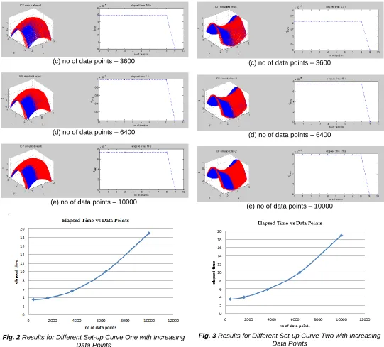
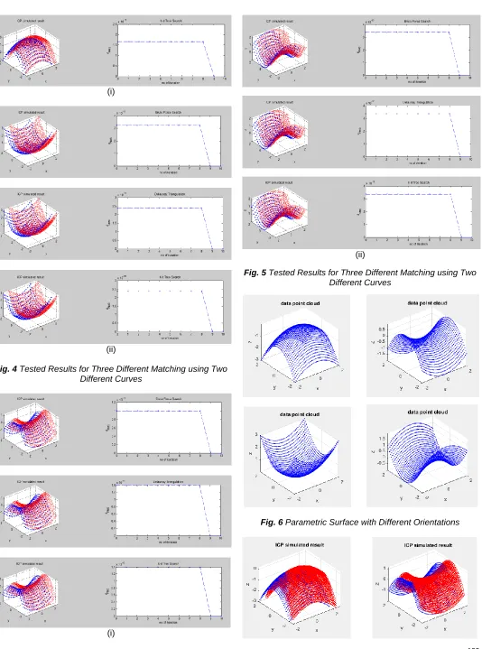
ESULTSIn this simulation, a cloud of points are used to represent any shape if the object surface is sufficiently densely sampled. Practically, these low level primitives can be obtained both directly from data measured by a 3D sensor and estimation from 2D-3D correspondence of image sequences from video camera. The model and data parametric surfaces are defined and registered using their geometry. By calculating transformation from one surface into the correspondence with the other, precise object localization and surface geometry can be obtained in 3D space. Using standard ICP implementation, Matlab code was written to perform on 3D point clouds. To analyze ICP convergence, initial transformation is varied in testing the simulation due to improper work of ICP for some specific shapes. For appropriate initial transformation, model and data point clouds can give global convergence. ICP is quite computationally demanding to identify the closest point for each object point at each iteration [1]. Processing time varies a lot depending on the number of points representing the object. As shown in Fig. 8, demonstration of elapsed time can be compared by using three different point set matching methods: Brute Force Search, Delaunay Triangulation and k-d Tree Search. Brute Force search is simple and can be expressed as O(N) for number of points N in point clouds. k-d tree is to divide the point clouds into groups according to their location. The nearest neighbor search is accelerated by conditionally excluding many points and thereby reducing the number of distance calculations. The creation of k-d trees and Delaunay triangulations takes considerable time while basically no preprocessing is necessary for a brute force search. The comparison on elapsed time for three different methods is shown in Fig. 8. Matching performance is tested with different number of points in data cloud. Tested results are shown in Fig. 2, Fig. 3, Fig. 4 and Fig. 5. Objects in the form of parametric surface shown in Fig. 6 are tested with
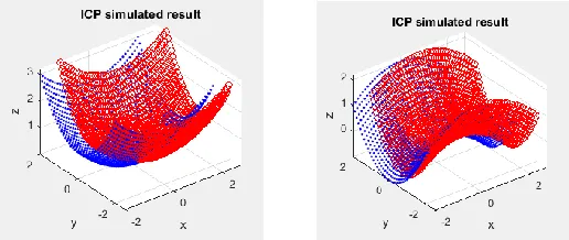
various initial orientations. The tested results are shown in Fig. 7. In these testing, number of iterations is fixed to ten to compare the elapsed time with number of increasing data points. The algorithm is terminated based on the number of iterations or the relative change in the error metric. In testing cases, the algorithm will converge quite rapidly. This may arise such as multiple local minima in the error metric, noise and outliers and partial overlap [10]. Multiple local minima means the algorithm may converge towards one of the local minima instead of the global minimum. Noise causes the error metric to never be zero. Outliers may cause faulty results. In partial overlap, the point clouds may not resemble the same parts of an object. The performance of these methods on matching is approximately the same from standard ICP algorithm.
5
C
ONCLUSIONSImportant issues of ICP algorithm are the speed of computation and the accuracy for 3D shape representation. The speed of the algorithm is crucial for many applications. When the number of points is very high, the basic ICP algorithm becomes very slow. For accuracy, a initial coarse transformation require globally estimate to allow the two views to get closer. Instead of searching dense point-to-point correspondences, suitable pre-alignment techniques may estimate practically the best matching between features extracted from the objects. Global features are a compact representation that effectively and concisely describes the entire object. In this comparison, matching methods focused on speed improvement for the closest point computation step. Another factor affecting the speed of ICP is the point-to-point or point-to-plane distance used. Not only computing the Euclidean distance between the data-point and model-point, but also point-to-plane distance computation is necessary to consider in objective function.
A
CKNOWLEDGMENTThe author wishes to express her gratitude to Yangon Technological University, for granting to perform this research work.
(a) no of data points - 400
101 (c) no of data points – 3600
(d) no of data points – 6400
(e) no of data points – 10000
Fig. 2 Results for Different Set-up Curve One with Increasing Data Points
(a) no of data points - 400
(b) no of data points – 1600
(c) no of data points – 3600
(d) no of data points – 6400
(e) no of data points – 10000
102 (i)
(ii)
Fig. 4 Tested Results for Three Different Matching using Two Different Curves
(i)
(ii)
Fig. 5 Tested Results for Three Different Matching using Two Different Curves
103 Fig. 7 ICP Results for Various Initial Data Point Cloud
R
EFERENCES[1] P. Besl, and N. McKay, 1992. ―A method for registration of 3-d shapes‖. IEEE Transactions on Pattern Analysis and Machine Intelligence, 14(2).
[2] V. Matiukas, D. Miniotas. 2011. ―Point Cloud Merging for Complete 3D Surface Reconstruction‖. Electronics and Electrical Engineering, No. 7(113).
[3] Timothée Jost and Heinz Hügli. 2002. Fast ICP algorithms for shape registration. Lecture Notes on Pattern Recognition.
[4] Micha Hersch et. al. 2011. Iterative Estimation of Rigid-Body Transformations, Springer.
[5] P. S. Manoj, et. al. ―A Closed-form Estimate of 3D ICP Covariance‖. IAPR International Conference on Machine Vision Applications, May 2015, Tokyo, Japan.
[6] S. Marden and J. Guivant. ―Improving the Performance of ICP for Real-Time Applications using an Approximate Nearest Neighbour Search.‖ Proceedings of Australasian Conference on Robotics and Automation, New Zealand, 2012.
[7] R. Boerner, and M. Kr¨ohnert. ―Brute Force matching Between Camera Shots and Synthetic Images from Point Clouds.‖ The International Archives of the Photogrammetry, Remote Sensing and Spatial Information Sciences, Volume XLI-B5, 2016.
[8] Bin Yang, Shuyuan Shang. 2012. Research on Algorithm of the Point Set in the Plane Based on Delaunay Triangulation. American Journal of Computational Mathematics, vol.2, pp. 336-340.
[9] Andrew W. Moore, ―An Introductory Tutorial on kd-Trees‖, PhD Thesis, Computer Laboratory, University of Cambridge, 1991.