Statistical Techniques for Improving the Repeatability of Automated ECG Interpretation

(1)

STATISTICAL TECHNIQUES FOR

IMPROVING THE REPEATABILITY OF

AUTOMATED ECG INTERPRETATION.

t .

I

*

Stephanie C. McLaughlin, B. Sc.

4

Thesis submitted for the degree of Ph.D.

To:

The Faculty of Medicine

University of Glasgow

The Research described in this thesis was carried out in the University

Department of Medical Cardiology, Royal Infirmary, Glasgow.

Stephanie C. McLaughlin

Signed:

k

(2)

ProQuest Number: 13834191

INFORMATION TO ALL USERS

The qu ality of this repro d u ctio n is d e p e n d e n t upon the q u ality of the copy subm itted.

In the unlikely e v e n t that the a u th o r did not send a c o m p le te m anuscript and there are missing pages, these will be note d . Also, if m aterial had to be rem oved,

a n o te will in d ica te the deletion.

uest

ProQuest 13834191

Published by ProQuest LLC(2019). C op yrig ht of the Dissertation is held by the Author.

This work is protected against unauthorized copying under Title 17, United States C o d e M icroform Edition © ProQuest LLC.

ProQuest LLC.

789 East Eisenhower Parkway P.O. Box 1346

(3)

LIST OF TABLES

TABLE

4.1 Mean, maximum and minimum ages of the 295 patients used to construct estimates of day-to-day variation.

4.2 Table of results for the amplitude of the R wave (mV) based on 295 patients.

4.3 Table of results for the duration of the R wave (msecs) based on 295 patients.

4 .4 Table of results for the amplitude of the ST segment (mV)based on 295 patients. 4.5 Table of results for the duration of the ST

segment (msecs) based on 295 patients.

6.1 Brief outline of the Glasgow scoring system for the detection of LVH.

6.2 Comparison of sensitivity between two methods. 6.3 Comparison of the sensitivities of the Discrete and

Smoothed programs.

6.4 Comparison of the specificities of the Discrete and Smoothed programs.

6.5 Repeatability of existing method (Day-to-day ECG recordings). 6.6 Repeatability of smoothed method

(Day-to-day ECG recordings).

6.7 Repeatability of existing method when comparing the severity of LVH (Day-to-day ECG recordings).

(11)

TABLE 6.8 6.9 6.10 6.11 6.12 6 .13 6 .1 4 6.15 6.16 6.17 6 .1 8

Repeatability of smoothed method when comparing the severity of LVH (Day-to-day ECG recordings). Comparing the inconsistent diagnoses of the existing and the smoothed methods

Repeatability of the existing method (Minute-to-minute ECG recordings). Repeatability of the smooth method (Minute-to-minute ECG recordings).

Repeatability of existing method when comparing the severity of LVH

(Minute-to-minute ECG recordings).

Repeatability of smoothed method when comparing the severity of LVH

Comparing the inconsistent diagnoses of the existing and the smoothed methods

(Minute-to-minute ECG recordings). Repeatability of the existing method (Split ECG recordings).

Repeatability of the smooth method (Split ECG recordings).

Repeatability of existing method when comparing the severity of LVH (Split ECG recordings). Repeatability of smooth method when comparing the severity of LVH (Split ECG recordings).

(12)

TABLE

7.1

7.2

7.3

7 .4

7.5

7.6

i“j r y

A comparison of existing and smooth methods of diagnosing ST Depression in lead II

(Day-to-day ECG recordings). 181

Repeatability of existing method when comparing the severity of ST Depression in lead II

Repeatability of smooth method when comparing the severity of ST Depression in lead II

Comparing the inconsistent diagnoses of the existing and smoothed methods for the day-to-day

ECG recordings (lead II). 183

Repeatability of existing method when comparing the severity of ST Depression in lead aVF

Repeatability of smooth method when comparing the severity of ST Depression in lead aVF

Comparing the inconsistent diagnoses of the existing and smoothed methods for day-to-day

ECG recordings (lead aVF). 184

(13)

TABLE

7.9

7.10

7.11

7.12

7.13

7.14

7.15

7.16

(Minute-to-minute ECG recordings). 186

(Split ECG recordings). 188

Repeatability of existing method when comparing the Inferior ST Depression-Index

(14)

I I TABLE 7.17 7.18 7.19 7.20 7.21 8.1 8.2 8.3 8.4 8.5

Repeatability of smooth method when comparing the Inferior ST Depression Index

Repeatability of existing method when comparing the Inferior ST Depression Index

(Split ECG recordings).

Diagnostic criteria in the Glasgow program for the identification of Q waves in the inferior and lateral leads (as of April 1990).

Repeatability of existing method (Day-to-day ECG recordings). Repeatability of smoothed method (Day-to-day ECG recordings). Repeatability of existing method (Minute-to-Minute ECG recordings). Repeatability of smoothed method

(15)

TABLE

8.6 Repeatability of existing method (Split ECG recordings).

8.7 Repeatability of smoothed method (Split ECG recordings).

9.1 Summary of results.

I

210

(16)

FIGURE 1.1 1.2 1.3 2.1 2.2 2.3 3.1 3.2 3.3 3.4 3.5 3.6 3.7 3.8

LIST OF FIGURES

The heart. 30

The ECG waveform. 32

Einthoven's triangle. 35

Distribution of the mean SV2 amplitude vs. Age

{based on 719 males and 584 females). 50

Distribution of the mean SV2 amplitude vs. Age (based on 719 male Caucasians and

205 male Chinese). 51

Mean SV2 amplitude vs. Age

{based on 719 males and 5 84 females). 52 Distribution of 1338 apparently healthy

individuals in the Glasgow Study. 57

Frequency Distribution of the R wave

amplitude in lead V5 (n=1338). 59

Discrete Upper limits of 'healthiness' for

the R wave amplitude in lead V5 (Males). 60 Plot of RV5 Amplitude vs Age in months (Males). 62 Plot of the fitted value vs. residual.

for the raw RV5 Amplitude. 62

Normal probability plot of the residuals for the

raw RV5 Amplitude. 63

Plot of Amplitude vs. Age (Males). 64

Plot of the fitted value vs. residual

(17)

FIGURE

3.9

3.10

3.11

3.12

3.13

3.1 4

3.15

3.16

3.17

Normal probability plot of the residuals

for the transformed data (i.e. VRV5). 65

Exact and Approximate upper 98 percentile

limits for (Males). 67

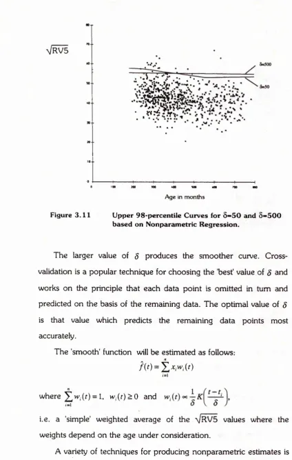
Upper 98-percentile Curves for 5=50 and 5=500

based on Nonparametric Regression. 70

A comparison of the upper limits of 'healthiness' calculated using a nonparametric regression

technique and a simple linear regression technique. 71 The smooth upper limit of 'healthiness' for the

square root of the R wave amplitude in lead V5 compared to the original discrete upper limit

(Males). 72

The smooth upper limit of 'healthiness' for the square root of the R wave amplitude in lead aVL compared to the original discrete upper limit

(Males). 73

The smooth upper limit of 'healthiness' for the square root of the S wave amplitude in lead V I compared to the original discrete upper limit

(Males). 73

Frequency Distribution of the QRS Duration

in lead V5. 74

Plot of QRS Duration in lead V5 vs. Age in months

(18)

FIGURE

3.18 Plot of the fitted value vs. residual for QRS

Duration in lead V5. 75

3.19 Normal probability plot of the residuals for QRS

Duration in lead V5. 75

4.1 QRS V5 Duration (msecs)

D ayl vs. difference between D ayl and Day2. 80

4.2 RI Duration (msecs)

D ayl vs. difference between D ayl and Day2. 81 4.3 Surface plot of the Approximate log-likelihood

function for the RV1 duration. 86

4 .4 Approximate 99% and 95% Confidence

Regions for (o,x) (RV1 duration). 87

4.5 Surface plot of the Exact log-likelihood

function for the RV1 duration. 87

4.6 Exact 99% and 95% Confidence

Regions for (a/c) (RV1 duration). 88

4.7 Surface plot of the Approximate log-likelihood

function for RV5 Amplitude. 89

4.8 Approximate 99% and 95% Confidence

Regions for (a,x) (RV5 Amplitude). 89

4.9 Negative P wave duration (msecs) in lead V I

Day 1 vs. Difference between Day 1 and Day 2. 91 4 .1 0 Transformed d." vs. Day 1

(19)

FIGURE

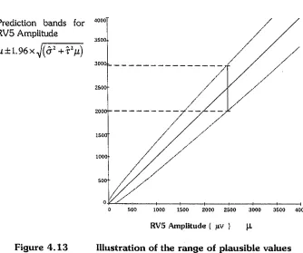
4.12 Illustration of the range of plausible values

for an observed RV1 Duration of 30 msecs. 96 4.1 3 Illustration of the range of plausible values

for an observed RV5 Amplitude of 2500mV. 97

4 .1 4 RII Amplitude {D ayl vs. D ay l-D ay 2 ). 98

4.15 Influence that x has on the sample mean. 101 4 .16 Influence that x has on the sample median in the

case where rt is even. 101

4.17 Plot of the unbounded influence function for RV5

Amplitude. 103

4.1 8 Example of a bounded influence function for RV5

Amplitude. 105

4.1 9 Surface plot of the Approximate log-likelihood function for RV5 Amplitude (taking account of

influential observations) (cf. Figure 4.7). 106 4.20 Approximate 99% and 95% Confidence Regions

for (c,t) (RV5 Amplitude) (taking account of

(20)

FIGURE

5.1 Discrete Score Function (Single threshold). 124

5.2 Discrete Score Function (Multiple thresholds). 125

5.3 The smoothed score function (Single threshold). 128

5.4 The smoothed score function (Multiple thresholds). 128

5.5 Smoothed score function for Lewis Index. 129

5.6 Smoothed score function for RV5. 130

5.7 Diagrammatic representation of the

Intersection Rule. 132

5.8 Smooth representation of the Intersection Rule. 133

5.9 Diagrammatic representation of the Union Rule. 134

5.10 Smooth representation of the Union Rule. 135

5.11 Contour plot of the discrete ST Score. 140

5.12 Surface plot of 5(xT,x2). 141

5.13 Surface plot of Sm*(jct,x2). 142

6.1 Diagrammatic representation of the discrete score function associated with P terminal

force in lead V I. 150

6.2 Diagrammatic representation of the smooth score function associated with P terminal

force in lead V I. 151

6.3 Diagrammatic Representation of the discrete score

function associated with Intrinsicoid Deflection. 152 6.4 Diagrammatic representation of the smooth score

(21)

FIGURE

6.5 Frequency Distribution of the Discrete LV Score {based on 136 Non LVH and 84 LVH cases) (See Table 6.1 for definition of Discrete Score). 6.6 Receiver Operating Characteristic Curve illustrating

the optimum cutpoint of 3.5.

6.7 Frequency Distribution of the smoothed LV Score (based on 136 Non LVH and 8 4 LVH cases). 6.8 Plot of D ayl scores vs. Day2 scores.

6.9 Frequency Distribution of the smoothed LV score (Day 1 recordings).

6.10 Plot of Minute 1 scores vs. Minute 2 scores. 6.11 Frequency Distribution of smoothed LV score

(Minute 1 ECGs).

7.1 Frequency Distribution of the smoothed ST Depression Index (Day 1 recordings).

7.2 Diagrammatic representation of discrete score function for Inferior ST Depression.

7.3 Diagrammatic representation of smooth score function for Inferior ST Depression.

7.4 Diagrammatic representation of discrete score function for Inferior ST Elevation.

7.5 Diagrammatic representation of smooth score function for Inferior ST Elevation;

8.1 Frequency Distribution of the smoothed Q wave index (Day 1 recordings).

(22)

FIGURE

8.2

8.3

8.4

8.5

8.6

Plot of Day 1 Q wave index vs. Day 2 Q wave index.

Day 1 ECG for a 54 year old male together with the interpretation obtained with the conventional program.

Day 2 ECG for the same 54 year old male as in Fig 8.3 together with the interpretation obtained with the conventional program.

Day 1 ECG for a 44 year old male together with the interpretation obtained with the conventional program.

Day 2 ECG for the same 44 year old male as in Fig 8.5 together with the interpretation obtained with the conventional program.

208

213

214

(23)

DECLARATION

I hereby certify that this thesis has been researched and written

entirely by myself and that it has not been submitted previously for any

degree.

Signed:

(24)

ACKNOWLEDGEMENT

I am deeply indebted to Professor P. W. Macfarlane for providing me with the opportunity of working in the field of electrocardiology and for all the genuine encouragement and assistance which he has enthusiastically given over the last few years.

Equally, I would like to express my thanks to Mr. T. C. Aitchison of the Dept, of Statistics for his unfailing support, guidance and friendship throughout the duration of this project.

This research would not have been possible without the help of many people. I would particularly like to thank Mr. B. Devine for all his patient programming assistance and Dr. F. Huwez for his helpful advice on various clinical aspects of the work. In addition, I am grateful to Mrs. C. Fullarton, Miss J. Kennedy, Mrs. K. McLaren and Mrs. M. Sneddon for their technical expertise in recording the numerous ECGs which were required.

I would also like to thank all my friends in the Departments of Medical Cardiology and Statistics and outwith the University for their helpful advice and assistance over the past few years.

(25)

SUMMARY

The electrocardiogram is a recording of the electrical activity of the heart. By convention, 12 separate leads are studied from which a diagnosis is made. This process of interpretation is a skill acquired by cardiologists over a period of years. During the past twenty-five years, computer assisted techniques have been developed to undertake such interpretations. It has been shown that if consecutive ECGs are recorded on a patient within several minutes, the computer diagnoses may differ because they are made independently of one another although all conditions remain unchanged. This discrepancy occurs when small changes in ECG measurements, from one recording to another, cause threshold values within the diagnostic program to be crossed, thereby producing conflicting diagnoses. The primary aim of the study described in this thesis was to develop techniques which would minimise such problems, thereby enhancing the repeatability of the ECG program developed in the Department of Medical Cardiology at the Royal Infirmary in Glasgow, whilst maintaining the heuristic framework of the diagnostic logic.

(26)

These limits have been replaced with continuous equations which were calculated on the basis of a sample of 1338 'normals' using simple linear regression techniques. It was thought that the use of such equations, which change smoothly and continuously throughout the age range, would alleviate the problem of subtle differences in ECG readings from recording to recording producing inconsistent diagnoses.

The second stage of the problem was to consider how to deal with discrete thresholds between normal and abnormal, whether such boundaries were continuous or not. Many of the diagnostic decisions throughout the program have, until now, been determined by whether the observed value of a particular ECG measurement has attained a specified discrete threshold. These decisions can be regarded as score functions for ECG measurements which take the value K if the threshold is attained, and 0 otherwise. No account has been taken of the proximity between the measurement and the boundary value. This 'all or nothing' strategy has m eant that an individual whose observed ECG measurement lies very close to, but below, a threshold value on one occasion and equally close to, but above, the same threshold value on a subsequent visit may receive two conflicting diagnoses.

(27)

the desired maximum score. In addition, the steepness of the new smoothed step was dictated by the amount of day-to-day variation in the particular ECG measurement under consideration.

Often, more than one criterion needed to be satisfied before appropriate action could be taken, so an algebra which would take account of combinations of criteria was required. Some basic mathematical rules such as the intersection rule and the union rule were used as building blocks upon which to construct such a system.

A database of 590 ECG recordings obtained on consecutive days from 295 patients (using no standardising procedures) was collected in order to estimate the amount of 'normal' day-to-day variation in the relevant ECG variables.

Preliminary investigations were undertaken with the aid of some simple exploratory plots of the data. These plots indicated that two models for day-to-day variation were required, each accounting for the fact that the amount of variation may or may not be dependent on the magnitude of the ECG measurement of interest. In most cases, the simpler of the two models was adequate, although in certain situations a slightly more complex model was required. Estimates of day-to-day variation were obtained for all the relevant ECG variables and subsequently used in the calculation of the new smoothed scores.

(28)

f

k

inferior ST depression was used as an indicator of the repeatability of the section of the program dealing with ST changes.

Repeatability was assessed in three ways:

1) on the basis of 660 ECGs which were recorded on two consecutive days from 330 patients;

2) using ECGs which were recorded within the space of a few minutes (without removing and subsequently replacing the electrodes) from 249 patients; and 3) using an artificial method of splitting the 330 day 1

ECG tracings into 2 digital representations.

In terms of overall repeatability, it was discovered that of the 330 pairs of repeat ECGs, 266 (81%) interpretations were completely in agreement with respect to the three previously mentioned diagnoses when the conventional version of the program was used. The corresponding numbers for the 249 pairs of minute-to-minute ECGs and 330 split ECGs were 222 (89%) and 3 0 4 (92%) respectively. Adopting the smoothing techniques in the conventional program increased the number of pairs of ECGs which were entirely in agreement in all three cases. Of the 330 pairs of day-to-day ECGs, 291 (88%) were in agreement, as were 236 (95%) and 315 (95%) of the minute-to-minute and split ECGs. There have therefore been substantial reductions in the percentages of pairs of ECGs exhibiting discrepancies. For example, the percentage of minute-to-minute ECG recordings producing inconsistent diagnoses has been reduced from 11% to just 5% which represents a 55% overall reduction in error. There were similar improvements for both day-to-day and split ECG recordings (37% and 38% overall reductions in error respectively).

(29)

verified via non-electrocardiographic means such as echocardiography, serum enzyme levels etc.), it was demonstrated that the conventional Glasgow program was perfectly repeatable in 2 95 of the 330 pairs of the day-to-day ECG recordings (89%), in 232 of the 2 4 9 pairs of ECGs which were recorded within the space of a few minutes (93%) and in 96% of the artificially split ECGs (i.e. 317 out of 330 tracings). Implementation of the smoothing techniques resulted in improved repeatability in ail three situations. For the day-to-day ECGs, the repeatability rose to 95% and the level of agreem ent from recording to recording was 98% for both the minute-to-minute ECGs and the artificially split ECGs, proving that the methods developed in this thesis are of benefit, even in situations when the level of agreement from recording to recording is reasonably acceptable.

The Glasgow program is long-established and has been associated with an acceptable diagnostic accuracy. In this respect, a study of the sensitivity and specificity of the new techniques compared to the old showed no significant difference in a group of 84 patients with LVH diagnosed by M-mode echocardiography.

(30)

CHAPTER ONE:

ELECTROCARDIOGRAPHY

1.1 INTRODUCTION.

Electrocardiography is the term used to describe the process which allows the electrical activity of the heart to be displayed in graphical form. The first human electrocardiogram (ECG) was recorded approximately one hundred years ago by Waller (1887) and since then, advances in modem technology have enhanced the field of electrocardiography and promoted its uses world-wide. Increasing popularity and demand for recordings of electrocardiograms led to research into the possible role of the digital computer as an analytic tool and the early 1960s saw initial automated analyses for both the 3-orthogonal lead and the 12 lead ECG (Pipberger et. al. 1960, Caceres et. al., 1962; Caceres, 1963; Stallmann et. al, 1961; Klingeman and Pipberger, 1967). Many benefits were anticipated, notably:

(i) the ability of computers to deal with the rapidly expanding demand for ECG recordings,

(ii) increased accuracy in the measurement of wave magnitudes and durations, and

(31)

1.2 ANATOMY

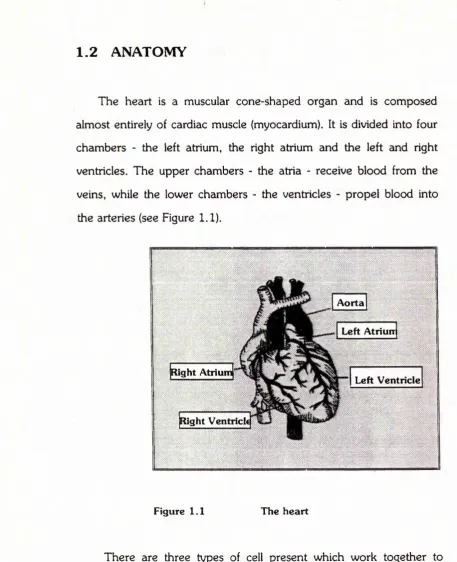
The heart is a muscular cone-shaped organ and is composed almost entirely of cardiac muscle (myocardium). It is divided into four chambers - the left atrium, the right atrium and the left and right ventricles. The upper chambers - the atria - receive blood from the veins, while the lower chambers - the ventricles - propel blood into the arteries (see Figure 1.1).

Aorta

Left Atriurr

Right Atrium'

Left Ventricle

Right Ventrick

Figure 1.1 The heart

(32)

bundle of His and the left and right bundle branches. Conduction then spreads through the specialised tissue in the ventricles known as ’Purkinje fibres' and into cardiac muscle itself. Stimulation of the muscle cells causes the mechanical contraction which is associated with each heart beat.

1 .3 THE FIRST ECG RECORDING

Contraction of the heart is associated with changes in polarity of the electrical charges on the surface of the myocardial cells. In the resting state, the cells are positively charged and when the cells are excited they enter a state of physical activity. This state comprises the electrical process known as depolarisation which changes the positive charge to a negative charge. Subsequent repolarisation then returns the cells to their resting state.

(33)

I

J

Lippmann’s electrometer and Burdon-Sanderson and Page (1878) who investigated the electrical activity of the tortoise heart.

Willem Einthoven developed a much more sensitive string galvanometer (Einthoven, 1901) which was designed with the purpose of recording the electrical activity of the heart. The electrical activity was detected by the quartz string in the galvanometer and the string's movement could be recorded photographically to make a tracing.

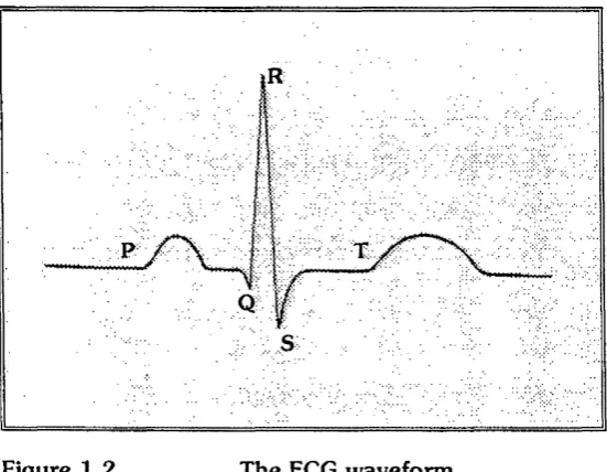
The ECG takes the shape of a waveform displaying characteristic peaks and troughs. Einthoven introduced the PQRST terminology to describe the deflections of the ECG waveform as illustrated below.

Figure 1.2 The ECG waveform

(34)

P wave

QRS complex ST segment

atrial depolarisation ventricular depolarisation

ventricular repolarisation {phase 2) ventricular repolarisation (phase 3) i wave

The P wave is of a smaller magnitude than the QRS complex since the atrial mass is less than the ventricular mass and hence repolarisation of the atria produces a relatively small deflection which by virtue of its timing is normally overwhelmed by the larger QRS

complex.

Several factors determine the magnitude and the direction of the deflections in the ECG, the most influential being the location of the electrodes on the body surface and the direction of the cardiac impulses in relation to the measuring system. By convention, if the depolarisation impulse travels towards the positive electrode an upward deflection will be recorded and vice versa.

There are two commonly used methods of displaying the electrical forces in the heart. Waller had first introduced a single dipole (1889) to represent the cardiac electrical activity and Einthoven and colleagues postulated that the m ean electrical axis of the heart could be represented by a vector (Einthoven, Fahr, de Waart, 1913). The first attem pt to form a vectorcardiogram (VCG), i.e. a loop that traced the direction of the resultant vector throughout the cardiac cycle, was published in an early paper by Williams (1914) who derived the cardiac vector from Einthoven's standard bipolar limb

(35)

f

\

leads. Through the following years, vectorcardiography evolved and Frank (1956) developed a 'corrected orthogonal-lead system' which essentially recorded three leads X, Y and Z measuring the component of the resultant cardiac electrical force in three mutually perpendicular directions. This is the most popular lead system for vectorcardiography and is still in use in various centres today.

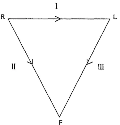
Bipolar leads were used by Einthoven et. al. (1913) to measure the potential difference between two limbs at points remote from the heart, hence the term bipolar limb lead. Electrodes were attached to the left and right wrists and to the left ankle to make the following connections :

Lead I Left Arm — > Right Arm

Lead II Left Leg Right Arm

Lead III Left Leg Left Arm

This may be represented mathematically as

I = El- Er

II - EF - e r

III = Ep - El

where EL, ER and EF signify the potential at the left arm, right arm and left leg, and I is the potential in lead I etc.

It follows that, at any instant in the cardiac cycle, I + III = II

(36)

i

effectively renders one of the leads redundant, allowing it to be calculated from knowledge of the other two.

Assuming that the right arm, left arm and left leg are arranged symmetrically around the heart and that the thorax represents a homogeneous conductor, the limb leads denoted I, II and III form an equilateral triangle with the heart lying approximately at the centre. This is known as Einthoven's triangle (Einthoven et. al., 1913).

R

F

Figure 1 .3 Einthoven's triangle

Investigation of the inhomogeneity of the thorax led Burger and an associate to redefine this triangle and to construct a scalene triangle - Burger’s triangle - of which Einthoven's triangle is a special case (Burger and van Milaan, 1946).

1908 saw the commercialisation of Einthoven's

(37)

Continuing research and collaboration resulted in Wilson's central terminal (Wilson et al, 1934). Electrodes were attached to the right arm, left arm and left leg as before and these were then averaged to form the reference or central terminal. This allowed an 'exploring electrode' to be used to record potential variation at each of the limbs as follows:

VR = _E_r_{" E}_wct

VL = _E_l_{‘ EWC}_t

VF - _E_f_{' Ewcr}

^WCT = i ( E R+ E L+ E F)

where ER, EL and EF are as before, EWCT denotes the potential at the central terminal which is relatively constant and VR, VL and VF denote the potentials measured at each of the limbs (Macfarlane, 1989b). Since the recorded potential effectively reflected potential variation at a single point because Ewcr is essentially constant, these leads were termed unipolar limb leads. When recorded in this way, the deflections were inconveniently small. However, slight modifications made by Goldberger (1942) to Wilson's central terminal produced augmented unipolar limb leads - denoted aVR, aVL and aVF - which essentially increase the voltages recorded by the unipolar limb leads by 50%, i.e.

aVR = - V R3

2

aVL = I V L

2

aVF = - V F3

2

(38)

Wilson's central terminal allowed a further six leads which recorded potential variation at single points on the chest to be introduced. These leads were called unipolar chest leads for obvious reasons and were initially denoted V I, V2, V3, V4, V5 and VE. Leads V I to V5 were derived from electrodes placed at designated areas on the chest and lead VE was positioned at the tip of the ensiform process (Kossmann and Johnston, 1935). Later, a committee of the American Heart Association published recommendations which were agreed upon by the Cardiac Society of Great Britain and Ireland on the positioning of six precordial leads V I, V2, V3, V4, V5 and V6 (Committee of the American Heart Association, 1938).

The combination of I, II, III, aVR, aVL, aVF, V I, V2, V3, V4, V5 and V6 forms the conventional 12-lead ECG which is the standard method for recording electrocardiograms virtually world wide.

A version of the waveform described previously is found in each of the 12 leads and the resulting ECG may therefore contain a vast amount of information. The ECG is usually interpreted in conjunction with any historical and clinical data which may be available.

1 .5 DIGITAL COMPUTERS

(39)

analysis of both the 12 lead and the 3-orthogonal lead ECG began in the late 1950s and rapid progress was being made by the early 1960s (Pipberger e t al, I9 6 0 , Caceres et. al., 1962, Caceres, 1963; Stallman et. al. 1961; Klingeman and Pipberger, 1967). These advances provided a stimulus for several other research groups (Bonner et. al., 1972; Macfarlane, Lorimer and Lawrie, 1971) and by the early 1970s automated methods being used by several teams yielded results which were in reasonable agreement with interpretations made by physicians. Such methods were implemented with the proviso that each automated ECG report be checked by medical staff before distribution. However, concern as to the repeatability of automated methods m eant that further research was required.

1 .6 DIAGNOSTIC PROGRAMS

Since the inception of automated electrocardiography two distinct methods for interpretation have been followed, each appealing to separate groups of researchers and benefiting from further developments. These methods are the statistical and the deterministic approaches to ECG classification, each having its own

advantages and disadvantages.

(40)

and more accurate than their deterministic counterparts (e.g. Klingeman and Pipberger, 1967). Initial work was done to distinguish between two populations (Eddleman and Pipberger, 1971; Goldman and Pipberger, 1969). Eddlemann used linear discriminant-function analysis with 15 ECG variables to diagnose correctly 88% of an independent test set of autopsy cases of myocardial infarcts. Goldman and Pipberger (1969) applied statistical techniques to a group of patients with conduction defects.

Cornfield et. al. (1973) used the established methodology in the multi-group situation which considered seven possible diagnostic categories, namely normal, anterior myocardial infarction, posterior myocardial infarction, lateral myocardial infarction, left ventricular hypertrophy, right ventricular hypertrophy and pulmonary emphysema.

A Bayesian approach was adopted whereby the posterior probability P(/lx) of an individual with ECG vector x belonging to diagnostic class i is calculated on the basis of the prior probability g,

of belonging to that class, i.e.

£ / ( a V ) « ; y=i

where

m - the number of possible diagnostic categories

f(x\i) - the conditional probability of x , given patient

belongs to i .

(41)

D eterm inistic m ethods were initially established by Caceres (Caceres, 1963). Such methods are built largely on experience and expertise which has been accumulating over many years, resulting in a logical path of decision rules which imitate the role of the cardiologist.

The development of both deterministic and statistical methods requires a substantial amount of data from different populations since it is known that ECG parameters vary according to age, sex and race. For example, Pipberger's AVA program which has been based on a male and war-veteran population is unlikely to perform in the same way on a group of young women.

(42)

the AVA program and the HP78 program, with overall performances being 80.3%, 72.8% and 63.3% respectively when diagnosing a variety of abnormalities (Willems et. al, 1986).

However, since multivariate techniques are typically based on the assumption that the primary diagnostic categories are mutually exclusive, the training set required to develop a statistical program with the ability to distinguish combinations of disease is likely to exceed the number of well-documented cases since each combination must be considered as a separate category (van Bemmel et. al., 1971). It is also apparent that the use of prior probabilities in statistical programs can influence the results. Indeed, the overall accuracy of the AVA program was decreased by 20% when prior probabilities were set equal for all possible categories (Pipberger et. al. 1975).

Deterministic methods appeal more to the end-user (i.e. the cardiologist) than statistical methods because they are more readily understood. Diagnostic criteria may also be selected on the basis of a knowledge of well-established electrophysiological processes. Deterministic methods are also reasonably flexible so that alterations to existing criteria can be implemented, and new diagnostic categories are easily added (Bailey and Horton, 1977; Kors and van Bemmel, 1990). Recently it has been demonstrated that, when cardiologist opinion is the gold standard deterministic methods have a higher accuracy than statistical techniques. However, when compared with the 'truth' (based on independent clinical evidence), statistical programs are more accurate (Willems et. al., 1991).

(43)

I »

this approach has not been widely used by clinicians and is therefore difficult to assess.

1 .7 THE CSE DIAGNOSTIC STUDY

As the number of commercially available interpretative ECG systems increased, so did the need for the development of evaluation methods which would serve to assess the diagnostic performances of the various ECG programs. Thus an international project was founded - the CSE Diagnostic Study - which aimed to establish common standards in quantitative electrocardiography. It was anticipated that, along with the assessment of diagnostic performance, exchange of information, improved co-operation between investigators, development of quantitative test procedures and improvements in measurement precision would also be achieved (van Bemmel, 1986).

The first stage of the CSE project was to develop standards for ECG measurements by evaluating measurement variability with respect to a reference based on results provided by referees. The second stage, the diagnostic study, aimed to assess the diagnostic performance of commonly used ECG interpretative programs by comparing their interpretations with those provided by cardiologists and with the 'truth' which was established on the basis of ECG- independent evidence such as catheterization, echocardiography and physical examinations (Willems et. al, 1991).

(44)

I I

ventricular hypertrophy, biventricular hypertrophy, anterior myocardial infarction, inferior myocardial infarction and combined infarction. Twelve different computer programs analysed the recordings - nine using the standard 12-lead ECG and three using the VCG. The recordings were also analysed independently by a panel of six cardiologists. The pilot study demonstrated several problems due to the different approaches used by the various programs (e.g. deterministic programs, statistical programs and programs based on fuzzy logic) and to the different terminology used by the centres. As a result, common CSE codes were introduced and each centre was required to apply a mapping scheme to produce the relevant code from the diagnostic statement. The performances of the diagnostic algorithms were compared using a statistical method outlined by Bailey et. al. (1988). Numerous preliminary results have been published (Willems et. al., 1987) but should be interpreted with caution given that they are based on a limited amount of data (Willems, 1988).

(45)

I

1 .8 THE GLASGOW PROGRAM

Since developments made throughout this thesis will be based around the structure of the Glasgow Program it is of relevance to describe the Glasgow approach briefly. Full details have been published elsewhere (Macfarlane et. al., 1990), while there will be an expanded discussion on relevant diagnostic criteria in subsequent chapters of this thesis.

The current 12-lead ECG program originated in 1977 after several years of developing and applying techniques for analysis of the 3-orthogonal lead ECG. The reason for this change was that mini computers became faster in the late nineteen seventies and the availability of microprocessors meant that multiple leads could be recorded simultaneously. Macfarlane et. al. (1980) developed a hybrid system around that time which allowed information from the 3-lead and the 12-lead ECGs to be combined.

(46)

f

\

The interpretative section of the program is deterministic in nature and considers all usual cardiac abnormalities. There are, for example, sections dealing with Conduction Defects, Ventricular Hypertrophy, Myocardial Infarction and ST-T abnormalities. The deterministic approach has been adopted largely on the basis of the disadvantages of the statistical approach previously described. Statistical programs are typically based on the assumption that the primary diagnostic categories are mutually exclusive and often this is not the case. Indeed, from over 30,000 ECGs which are recorded in Glasgow Royal Infirmary each year, there may be innumerable combinations of diagnostic statements. The training set for a statistical program which will allow identification of many combinations of cardiac abnormality is impractical since vast amounts of data representing each category will be required in addition to data representing each subdivision of the population (sex, age, race). Furthermore, manipulation of prior probabilities can often lead to misleading diagnostic results. Finally, clinical information may be used more easily in deterministic programs and the output from such programs is more acceptable to clinicians.

1 .9 SERIAL CHANGES

It is important to be able to examine the serial changes in an ECG over time since this will allow monitoring of the progression of a particular disease.

(47)

Selected measurements pertaining to the detection of sequential changes in myocardial injury were stored and criteria produced. The analysis of day-to-day and beat-to-beat variation in a group of normal serial ECGs (Cawood et. al., 1974) provided knowledge of the amount of variability which could be construed as 'normal' and the criteria for the detection of sequential changes were thus established.

Currently, in the Glasgow program, three ECGs are compared for an individual in any given year (Macfarlane, 1989c). The primary record is the first recording and the other two are those most recent prior to the current ECG. Where ECGs are compared with earlier recordings there will be some indication of whether there have been significant changes or not.

1 .1 0 DAY-TO-DAY VARIATION

(48)

without replacing the electrodes. Of the 40 5 pairs of ECGs which were considered, type A statements (i.e. statements referring to conditions which can be verified via non-electrocardiographic sources such as echocardiography and physical examination) were reproduced in 93% of cases. This reproducibility is superior to that obtained by human readers.

In 1974, Bailey and his associates suggested a method of testing the reproducibility in ECG program performance which was independent of the clinical accuracy of the program (Bailey et. al., 1974). Instead of using two consecutive recordings from each patient, two digital representations from the same tracing were obtained. Initially the analogue data sets were collected at 1000 samples per second from which two data sets were extracted representing the same analogue data only this time digitised at 500 samples per second and separated in time by one msec. The performance of four programs was assessed and results reported. The IBM (1971) program was superior both to version D of the PHS program and to the Mayo Clinic program of 1986 exhibiting identical diagnostic statements in 76% of tracings compared to 43.3% and 60% for the PHS(D) and Mayo Clinic programs which were available at that time. Analogue filtering had the effect of increasing the percentages of identical statements to 79.7% and 49.8% for the IBM and PHS(D) programs respectively. The fourth program which was examined in this way was version 3,4 of Pipberger's automatic vectorcardiographic analysis (AVA) program (Bailey, Horton and Iscoitz, 1976). Identical readings were observed in 82.4% of 217 filtered ECGs.

(49)

reproducibility of any diagnostic program is the reproducibility of the ECG (Tuinstra, 1986) and noise and measurement errors may mean that deterministic programs may be more susceptible to repeat variation than their statistical counterparts (Willems, 1977). Bailey and his associates stressed the importance of reproducibility testing of ECG interpretative systems (Bailey et. al, 1976) and this remains a fundamental issue when assessing and evaluating diagnostic programs.

(50)

CHAPTER TWO:

DIFFERENCES IN ECG WAVEFORMS.

2 .1 INTRODUCTION.

Despite the many advantages gained through automated interpretation of the electrocardiogram, there remains cause for concern about the lack of repeatability of such techniques. By adopting a computerised approach to the analysis of ECGs, certain sources of errors have been minimised or indeed eliminated. For example, human error is removed and accuracy in wave measurements increased (Macfarlane and Lawrie, 1974). However, it can happen that on two consecutive clinic visits two conflicting ECG diagnoses may occur when there has been no clinically significant change in the pattern of the ECG waveform. The reasons for this are plentiful.

Before considering possible causes of repeat variation it is perhaps of value to mention several factors which can influence the appearance of the ECG from one individual to another.

2 .2 DIFFERENCES IN ECG APPEARANCES.

(51)

factors have been taken into consideration, measurements such as height and weight provide little additional information on variability.

2 .2 .1 D ifferences due to sex.

Young adulthood appears to be the period in which sex differences in the ECG become obvious, such differences perhaps being due to the higher fat content of females and the presence of breast tissue, resulting in lower voltage amplitudes (Macfarlane and Lawrie, 1989d). Differences in the SV2 amplitude between male and female Caucasians are illustrated in Figure 2.1.

SV2 (mV)

2

-1 —

i

1

II

1 8 -2 9 8 0 -8 9 4 0 - 4 9 50 +

Age

□ Male

□ Female

Figure 2.1 Distribution of the mean SV2 amplitude vs. Age

(52)

2 .2 .2 D ifferences due to race.

Differences in the magnitude of ECG variables can also be observed when comparing races. The following histogram (Figure 2.2) illustrates how the amplitude of the S wave in lead V2 varies between Caucasians and Chinese (Chen, Chiang and Macfarlane,

1989).

SV2 (mV)

1 8 -2 9 3 0 -8 9 4 0 - 4 9

Age

a Chinese

a Caucasian

50 ♦

Figure 2 .2 Distribution of the mean SV2 amplitude vs. Age

(Based on 7 1 9 male Caucasians and 2 0 5 male Chinese)

2 .2 .3 D ifferences due to age.

(53)

f

SV2 (mV)

Figure 2 .3

Sex and race are used as categorical variables in deterministic programs. This means that they are separated into categories for diagnostic decision making, normally consisting of a small number of classes {i.e. two for sex and two for race when considering Caucasian and Chinese only). Age, however, is a continuous variable which until now has been categorised into several mutually exclusive groups by all deterministic programs, e.g.

18-29, 30-39, 40-49, 50+

U pper limits of normality for ECG variables are usually constructed for each age group, stratified by sex and race, resulting in several distinct categories into one of which a particular individual will belong.

The above categorisation of age may cause problems if, between consecutive recordings, an age threshold has been crossed. Different upper limits of normality apply to the magnitude of the S wave in lead V2 for adult males under 30 years than for those aged between 30 and 40 so that if a particular individual's SV2 measurement has not changed from one clinic visit to the next but his 30th birthday

- a - Male

•■■*¥■■■ Female

1 8 -2 9 3 0 - 3 9 4 0 - 4 9 5 0+

Age

Mean SV2 amplitude vs. Age

(based on 7X9 m ales and 5 8 4 females) 2

1

(54)

I I

has occurred in the interim, it is possible that his ECG may be considered as normal on one occasion and abnormal on the next. This is one contributory factor to the problem of repeat variation and arises as a result of the discontinuous nature of many boundaries.

It is clearly unlikely that an individual's ECG waveform will be completely identical from one recording to the next. There will typically be small, clinically insignificant changes in wave amplitudes and durations. Regardless of how minute such changes may be, conflicting computer diagnoses can occur if discrete boundaries are crossed and this phenomenon, combined with the age-related discontinuities, forms the crux of the problem of repeat variation.

2 .3 DAY-TO-DAY VARIATION.

Variation in the PQRST amplitudes and durations can potentially lead to a lack of repeatability in computer diagnoses from one ECG recording to another and this naturally gives cause for concern. Knowledge of the causes of day-to-day variation allows an experienced cardiologist to report no significant change between consecutive recordings although a method by which such variation may be quantified would prove appealing. On the other hand, cardiologists are not infallible. The CSE diagnostic study found that the median repeatability of cardiologists when given the same ECG on two separate occasions was 81.8% (Willems et, al., 1991).

(55)

Simonson first addressed the question of day-to-day variation and emphasised the need for knowledge of such variation in order that serial electrocardiography be carried out (Simonson, Brozek and Keys, 1949). He suggested that eating a meal between recordings may alter the ECG significantly and provided measures of the amount of variation exhibited between eleven consecutive recordings taken over a period of two months on twelve normal young men.

Graybiel and colleagues demonstrated the effects of inhalation of tobacco smoke on the ECG (Graybiel, Starr and White, 1938). Drinking iced water between recordings has also been shown to alter ECG appearances (Sears and Manning, 1958).

Electrode placement is another cause of repeat variation since varying distances between the electrode and the heart will result in different ECG potentials and durations being recorded. It is therefore important that due care and attention is given to the placing of the electrodes when ECGs are being recorded.

Day-to-day variability can be reduced by the order of 25% when electrode positions are marked between recordings. Willems et. al. (1972) demonstrated such a reduction when comparing 3-orthogonal lead electrocardiograms which were recorded on individuals whose electrode positions were marked with a coloured skin marker and on those whose electrode positions were unmarked. Although repeat variation was reduced to a certain extent with such an approach, it was not eliminated.

(56)

and there still remains sufficient concern as to the other factors contributing to repeat variation.

2 .4 SUMMARY.

The sources of variation in ECG appearances which have been described can be divided into two categories

-a) 'between-individual' variation and b) 'within-individual' variation.

'Between-individual' variation will arise due to the fact that many ECG variables have been observed to vary with sex, race and age. Many ECG-analysis programs can deal with the former type of variation by stratifying by age, sex and race although using age as a discrete variable can give rise to a lack of repeatability.

(57)

CHAPTER THREE:

SOURCES OF REPEAT VARIABILITY

IN THE ECG:

A gc-catcgoriscd 'normal ranges'.

3 .1 INTRODUCTION.

In the previous chapter attention was given to the fact that upper limits of normal for selected ECG variables are stratified by age, sex and race. The reason for this is that many ECG measurements differ across sub-groups of the population and it would be inadvisable to make use of the same criteria for young male Caucasians as are used for older female Chinese.

Having been stratified by race and sex, many limits are usually categorised by age and the problems arising from such a procedure have already been discussed. While these limits will remain stratified by race and sex, it is appealing to make use of the continuous nature of age in providing smoothed age-related upper limits of normality where appropriate.

3 .2 BACKGROUND TO SAMPLE SELECTION.

(58)

the smaller group (which will be more accessible than the target population) are to be extrapolated to the larger population.

Several approaches to population sampling have been identified. Macfarlane et al. (1985) opted to cover a variety of occupations in order that both sedentary and manual workers were included. To achieve this, volunteers from several departments in local government in the region of Strathclyde were sought. The distribution of the

1338 subjects may be seen in Figure 3.1.

400

Frequency

300

200

100

0

Figure 3.1

It can be seen that there is a predominance of younger persons in this sample, presumably because they are more willing to volunteer for screening. This can be attributed to the fact that the probability of finding any abnormality of a cardiac nature will be lower in the younger age groups than for older people. It is also clear that there is a large difference in the number of males and females in the 30+ age

a Males

a F em ales

18-29 30-39 4 0 4 9 50+

Age C ategory

(59)

categories since many women opt to leave employment at this stage in order to start a family (Macfarlane, 1989d).

Any form of extrapolation from this sample must be questionable since the sample of individuals obtained is not entirely representative of the population in general. In particular, the subgroups specifically thought to be 'at risk', typically the older groups, are not as well represented as the younger subgroups. Therefore any inferences which may be made about such groups should be interpreted with caution although, hopefully, the smoothed age-related upper limits of normality that are produced from this data will not be biased, merely better estimated for the younger ages and for males.

3 .3

THE CURRENT SITUATION:

3 .3 .1 B asic A ssum ptions.

(60)

mean ± 2 standard deviations.

If the underlying distribution of a particular variable is non- Normal, then it may be possible to transform the variable to achieve approximate normality. As a last resort, certain situations may necessitate the use of nonparametric methods of inference to estimate 'normal' or 'healthy' ranges. Such methods do not require strong assumptions as to the underlying distribution which generated the data but are often inferior in providing strong inferences.

It has been established (Simonson, 1961) that the distribution of many ECG variables is skewed so that the normality assumption does not apply. For example, the unconditional distribution of the R wave amplitude in lead V5 is skewed to the right (see Figure 3.2).

Frequency

RV5 (mV)

Figure 3 .2 Frequency Distribution of the R wave

amplitude in lead V5 (n -1 3 3 8 )

'Healthy' ranges for the raw age and sex categorised data collected in Glasgow should therefore not be presented as mean ± 2 standard deviations. Instead, 2% of observations were excluded from

(61)

100-percentile range is used in many electrocardiographic studies instead of the standard 95% range and there is no special reason for opting to exclude 2% of values rather than 2.5% other than the preservation of continuity.

3 .3 .2 D iscrete Upper Limits.

Upper limits of ’healthiness' for many param eters of interest have been constructed on the basis of the 96% range of the data {Macfarlane, 1989e) and an example of how this limit varies over age and sex for the R wave amplitude in lead V5 can be seen in Figure 3.3.

5 0 0 0 n

---RV5 400e“---[ (|xV)

3 0 0 0 - 1--- [

2000

-I00

Q-o4l 1---1---1

---2 0 3 0 4 0 5 0

Age in years

Figure 3 .3 Discrete Upper limits of 'healthiness* for

the R wave amplitude in lead V5 (Males)

(62)

values are a potential source of lack of repeatability and it is therefore of interest to replace such discrete upper limits of normal with limits which change continuously and smoothly with' age.

3 .4 SMOOTHING OUT DISCRETE LIMITS:

The u se of linear regression.

As an initial step in our main aim of predicting the upper limit of 'healthiness' for a particular ECG variable x, we specify a model to describe the dependence of * on age t . The simplest possible model is a linear regression where the conditional expected value of x

depends linearly on t and the variability about such a linear relationship is constant. As in the previous section, the assumption of normality (in this case for the conditional distribution about the expected value) is questionable, so suitable transformations were investigated.

As an example, normality of the conditional distribution of the R wave amplitude in lead V5, given the age, will be assessed.

(63)

500&

RV5

m

4000-

3000-2000

-1000

-Figure 3 .4

i i r

0 100 200 300 400 500 600 700 800 900 1000

Age in months

Plot o f RV5 Amplitude vs Age in months (Males)

After applying standard linear regression techniques it is possible to plot the residual values against the fitted values (see Figure 3.5) to assess the adequacy of the linear model.

Residual

3000-2000

-1000”

-loocr

-2000

’* /- W'- V V. ■

* '^ ..t'■ * *»*■ t v »s *j

•_, _{'.s .} ₄

n i i i i i i i i

1300 1400 1500 1600 1700 1800 1900 2000 2100 2200 2300

Fitted Value (]xV)

Figure 3 .5 Plot of the fitted value vs. residual

for the raw RV5 Amplitude.

Statistical Techniques for Improving the Repeatability of Automated ECG Interpretation