http://www.sciencepublishinggroup.com/j/ijdsa doi: 10.11648/j.ijdsa.20170301.12
Project Evaluation from Application to Econometric
Theory: A Qualitative Explanation of Difference in
Difference (DiD) Approach
Muhammad Ateeq-ur-Rehman
1, 21
Gutenberg School of Management and Economics, Johannes Gutenberg University Mainz, Mainz, Germany
2
Lahore Business School, the University of Lahore, Lahore, Pakistan
Email address:
To cite this article:
Muhammad Ateeq-ur-Rehman, Project Evaluation from Application to Econometric Theory: A Qualitative Explanation of Difference in Difference (DiD) Approach. International Journal of Data Science and Analysis. Vol. 3, No. 1, 2017, pp. 5-12.
doi: 10.11648/j.ijdsa.20170301.12
Received: September 1, 2016; Accepted: April 14, 2017; Published: April 26, 2017
Abstract:
The main objective of this study is to show the importance of the Difference in Difference (DiD) method and its applicability in the field of human and social sciences. The DiD method is one of the famous tools in econometrics to investigate the causal effect of the policy before and after treatment or policy. Why difference in difference method is most important in these days? Because the traditional methods requires more instructions as compare to DiD method which is easier and applicable without randomization of the data. The difference is compared with treated and non-treated group in two time’s period model with the same unit of data. The first difference removes the time-invariant factors while Difference in Difference removes the time-variant factors of the model and the remaining statistic shows the original impact of the treatment or policy.Keywords:
Econometrics, Difference in Difference, Policy1. Introduction
The main objective of the development policies are to change the economic outcomes injecting different economic shocks to the economy. Which factor should be changed to achieve the required output and which factor should be controlled?, is the major concern of the strategic policy makers. However, performance-based policy plays an important role in the economy and economic differences after policy shocks can be measured through econometric tools. Difference-in-Difference (DiD) is one of the important methods to evaluate the policy result and is being mostly used in social and economic sciences. In general, Difference-in-Difference approach measures the average difference of two comparable groups before and after policy implementation while the policy is considered effective if comparative group difference is decreased. Specifically, in the situation of nonrandom and discontinuous data type, the difference in difference method can be more applicable and favorable to generate the required results [1]. Generally, different four groups are taken into analysis and three of
those are not treated while the one treated or enrolled group is analyzed to investigate the policy effect [2]. By assumption, the required average outcomes cannot be achieved without treatment effect. The controlled (untreated) and treated groups are analyzed critically according to pre and post-treatment period. The linear parametric model shows the different time-variant and time-invariant coefficients of interest but it is assumed that the relative coefficient of interest is not correlated with other individual observation. In addition, the mean difference of treated and untreated group before and after policy decides the impact of intervention. Difference in difference approach measures the efficiency and affectivity of the policy in repeated cross-section panel data type [3].
binary nature to check the coefficient of interest known as difference-in-difference estimator. Why difference in difference method is most important in these days? Because the traditional methods requires complex procedures as compare to DiD method which is easier and applicable without randomization of the data. In the first difference the time invariant behavior, within the same group, is removed while in the double difference, the time variant behavior is removed from the both group. Meanwhile, the main result shows the original change because of the policy intervention. Thus the DiD removes not only the selection bias but also eliminate the time variant bias and the rest of the change shows the counterfactual [1].
The contemporary study presents a brief view of DiD and explain the common approach and methodology of the method. In addition, it explains the importance of the DiD and the related issues as well referring the paper written by [4]. The major strengths and weaknesses of the method are also the relative part of the contemporary research work.
The outline of the paper is as follow; Section 2 discusses the historical understanding with some interesting application and also explains the reasons and the importance of the DiD approach. Section 3 gives a detailed view of the method with example and some specific issues. The critical assessment of the method is also taken into account in the same section. Section 4 concludes.
2. Theoretical Background
Difference in Difference method is a popular tool to find the causal effect of the public intervention on the treated group. Firstly, in order to find the reason of death because of impure water in the center of London. By applying Difference-in-Difference method, the study discovers the contaminated water was the main reason of high death rate
[5]
. The same method is also used to investigate the impact of the change in the law regime on the working stoppage in the United States [6]. Another study applied the same techniques in economics and investigates the impact of minimum wage law on the employees in Oregon comparing with other employees [7]. Consequently, difference in difference approach has also been applied to discover the impact of the price on the sandwich sale comparing the treated and non-treated group. In this regard, the method removes all trend and constant behavior of the sale and the remaining part clearly states the real impact of the price on the sale [8]. Subsequently the same method is applied to explore the effect of trade openness on the productivity and wages in Uruguay. By introducing ‘’Southern Common Market (MERCOSUR)’’ agreement, the trade openness increases the productivity of the firms in Uruguay and reallocation strategy of the resources also increases the wage level due to MERCOSUR law of trade in Uruguay [9]. Difference in difference approach is used to investigate the illegal behavior of the ‘Marshfield clinics’ in Wisconsin. The comparison of two groups, involved in illegal conspiracy and not involved in unlawful behavior
[10]. In addition, the same method is applied in management field and finds the impact of merger on the stock price using the data of gasoline companies in Spain [11]. Another study also uses the same approach to investigate the relation of environmental policy with the carbon level in the industry [12]. The study finds the relation of water with child mortality using the difference in difference approach. By comparing the group using publicly provided water, with the group, using privately water supply, a less mortality child rate is found with the group using privatized water scheme as compare to the controlled group not using privatized water [4]. Last but not least, another study applies the difference in difference method analyzing the impact of financial assistance (Progresa) on the child enrollment at primary and secondary school in Southern Mexico. The study finds that the impact of the intervention is more on girls as compare to boys [13]. The literature shows the importance of difference in difference approach academically and practically in different fields.
2.1. The Method
Difference in Difference method is not only specific to the field of economics but also can be applied to the other field of sciences as discussed in the literature. It is the technique to estimates the mean differences between two groups keeping in view that one of the group members is exposed with treatment while the other one is not. The method does not follow the random sampling techniques and therefore known as the ‘quasi experiment method’ or ‘natural experiment method’. Difference in Difference approach just explains the effect of the outer shocks on relative outcome comparing with the unaffected observations having same characteristics. The following steps are taken into account when the method is applied.
2.2. Definition of the Variables
The two groups are defined having somewhat similar characteristics before treatment and this way of selection can remove the biasness from the model while one of them is exposed for the treatment. In addition, the similarity between both groups before treatment is necessary for the validity.
2.3. Time Specification
Time specification is the more important element in this method and time period with same unit is replicated when treatment is exposed to one of two groups. The time period when intervention is not exposed, is known as ‘before’ or ‘baseline’ while the ending time of the intervention is known as ‘after’. Both time periods are compared relative to policy matter and the difference is captured through DiD.
2.4. Computation of the First Difference
2.5. The Final Outcome (DiD)
The ending part of the method is a ‘’counterfactual’’ of the two groups and again the difference is calculated from the first differences of the treated and untreated group. In first difference, the time invariant factor is removed and in the double difference the time variant factor is removed with in two groups. The rest of the part shows the original effect of the policy on the treatment group. So these steps show that how the method work and what are the steps necessary to run the method.
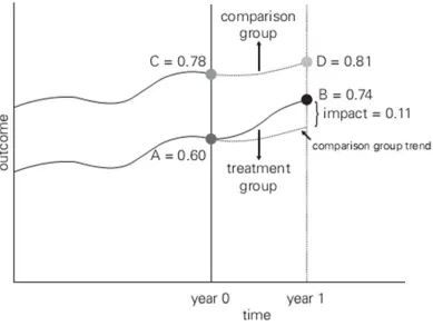
In Appendix (Figure 1), a conceptual explanation is given to illuminate the difference in difference approach briefly where the outcome of the group (A and C) is on the baseline period. This scenario shows the outcome of the both group before the treatment while D and C show the outcomes of treated and untreated group after a specific time period. The line between point A and B clearly shows the trend in comparison with untreated group which shows that the difference between B and D is less as compare to A and C. In addition, Appendix (Figure 2) shows in detail understanding regarding DiD. In the first column the variables names are categorized and second column shows the post-intervention facts of the two different periods while the third column shows the difference within the group. The DiD shows the actual change because of intervention.
The first difference of treatment and controlled are given as (B-A= 0.14) and (D-C= 0.03) respectively in the last column of the Appendix (Figure 2). In the end of the last column, Difference in Difference is calculated as shown in the equation (1).
= − − − (1)
= 0.74 − 0.60 − 0.81 − 0.78 = 0.11
This is the approach of the method through which the actual change is calculated and also known as mean causal effect.
3. Assumptions of the DiD Model
Cameron and Trivedi (2005) state the following assumptions of the DiD model.
Assumption 1: ‘Common trend’ or ‘time effect’ remain same for treated and control group
Assumption 2: ‘Bias stability’ or ‘Composition stability’ in treated and untreated group remains same if cross-sectional data is used
3.1. Common Approach
3.1.1. Linear Formulation
The linear regression model is widely used to perform the same result as shown in Appendix (Figure 3) and linear form of the model is shown in equation (2)
= + + + . + (2)
Here, Y shows the final outcomes of the model while is
the dummy variable and it takes value 1 if the dummy variable is in the treated group and ‘0’ otherwise. is the time dummy and it takes the value 1 in the post treatment stage and ‘0’ in the pre-treatment stage . The most important coefficient of interest in the equation (2) is which shows the result of interaction term of time dummy ( ) with treated group ( ) after intervention. In addition how is calculated is also shown in equation (3) which shows the back end procedure of the coefficient of the interest and it is just difference of the mean difference of controlled and exposed group. Thus it is called the difference in difference calculated by simple linear regression where the individual sample takes only two value ‘0’ or ‘1’ which prove the linearity of the model.
= , − , − , − , (3)
3.1.2. Non-Linear Formulation
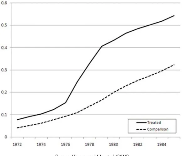
There are some outcomes which cannot be analyzed using linear model and then a nonlinear model is applied to investigate the coefficient of interest. Thus DiD method is applied combining linear index with nonlinear function through probit and logit model but the common trend is not same. In simple linear model the unobserved heterogeneity remain constant and consistent over time while in nonlinear model it remains inconsistent because of variation in group specific differences. In addition, the nonlinear model is applied when experimental data is not available and the treatment effect is not same with in the sample group as shown in Appendix (Figure 4). It shows the trend of the treated child ratio compared with controlled group as an example of non-linear group.
Different statistical models are applied to find the distributional form of the model and the most popular models are probit and logit.
In probit model, standard normal distribution function is estimated through linear index of the dummy variables while in logit model, cumulative distribution function is derived from different subsamples. The general idea is to find the impact of the treatment or policy on the different subgroups of the sample as shown in the Appendix (Figure 5). The probability score is between 0 and 1while the common trend or fixed effect is removed by taking difference and the remaining difference of the distribution is known as the policy effect.
4. Evidence
municipality in Argintina. [4]. Another study identified the change using difference in difference approach proving that the change is not related to another unobserved time-variant and time-invariant heterogeneity which was the main objective of the study. The difference was observed around 8% which clearly states the impact factor of the intervention on the mortality rate. First of all the study shows that overall people have become more health conscious and they prefer to get pure water in order to protect the life. In Appendix (Figure 5 and Figure 7) show the general facts about the share of households connected to the water and sewerage all around the world and it shows that the poorest part of the household is shifted to the pure water area or privatized water supply area as compare to the richest ones. In the context of Argentina the same case is with poor people and they shifted themselves to the area where private companies offer the pure water. Difference in difference results in Appendix (Figure 6) shows the significance of the method and a positive effect (0.018 and 0.042) shows that people shifted from local water municipalities to privitazied water municipalities in Argentina.
The study also checks the trend of the mortality rate before the privatization policy as shown in Appendix (Figure 3). Before 1995, the average trend shows that mortality rate in privitized and non privitized municipalities was same but after the intervention, the death rate in privatized municipalities decreased faster than non privatized one in Argintina which perfectly remove the common trend and provide a solid background in order to genreate the result using DiD. It also uses the data to check the economic shock (time variant factors) on the mortaliy rate but the results show that other factors have no cause to mortality rate as shown in Appendix (Figure 8). The only one reason to decrease the mortality rate was the intervention as shown in the first row of the Figure 8 with different time variant and covariant factors[4].
By analyzing the result shown in Appendix (Figure 8), it is clear that the interevention played an important role to decrease the mortality rate if the other factors are not controlled. Because of hetrogenous response from different municipalities, comparison problem and different observation create a biasness in the model. The matching method is used to resolve the problem of selection and covariant source of biasness from the model. The common support region eliminate the selection biasness and reweighting the controlled group after the selection biasness eliminates the second source of biasness which is also known as distributional biasness. The reweighting techniques again find the difference in difference which is also known as the generalized difference in difference technique. In this technique, the coefficient of interest is calculated given the time invariant factor of the treatment group in the mode and the similar controlled group is matched with treatment group before intervention [4].
The scientist establish the probability distribution function using logit model and find the common area of the distribution. At last the genrealized difference in difference
method is applied by reweighting the area of the distribution as shown in Appendix (Figure 8) from column 4 to 7.In the last column, the generalized difference in difference shows that the intervention cuses to decrease the mortality around 9%.
Difference in difference method is a famous tool now days to find the impact of the policy but it is impossible to fully disclose an uncertainty by the same method. The attractive point of this method is just to analyze the situation before and after intervention. The method is also a good tool to tackle the non-experimental data type problems to investigate the causal effect of the policy. Contrary to that, it is not possible to control the time variant and covariant factors which is a debatable issue related to that method. Because of this problem, the parameters become inconsistent with in the model. Therefore the best and consistent coefficient depends upon the true value of the uncertainty with in the model. Consequently, the heterogeneous time trend of different region can become a reason of inconsistent coefficient of uncertainty. In addition, if the common trend is not constant and it has also a lag relation of more than two time’s period then coefficient of interest does not show the true picture of the scenario. So the counterfactual part of the outcome cannot show the true value of the parameters because of mentioned reason and then the assumption can be tested for further analysis.
5. Conclusion
The difference in difference method is one of the famous tools in econometrics to investigate the causal effect of the policy. Why difference in difference method is most important in these days? Because the traditional methods requires more rules as compare to DiD method which is easier and applicable without randomization of the data. In the first difference the time invariant behavior, within the same group, is removed while in the double difference, the time variant behavior is removed from the both group and the result shows a pure change because of the policy intervention.
The historical background shows the importance of the method and its applicability in the different field of human and social sciences. DiD method follows some steps to generate required outcomes in which two groups are compared to check the effectiveness of the policy. The difference is compared with treated and non-treated group in two time’s period model with the same unit of data. The first difference removes the time-invariant factors while Difference in Difference removes the time-variant factors of the model and the remaining fact shows the original impact of the policy while the method is applicable to both nonlinear and linear functional form of the model.
ineffectiveness of the other shocks with in the model as shown in Appendix (Figure 8). At last further investigation of
the assumption of the model can be tested in order to generate the consistent parameters of the model.
Appendix
Source: Gertler, et. al., (2011)
Figure 1. Graphical Explanation of DiD.
Source: Gertler, et. al., (2011)
Source: Havnes and Mogstad (2010)
Figure 3. Child Coverage Rate (1972-1985).
Source: Gertler and Martinez accessed from (www.google.com (2012)).
Figure 4. Nonlinear Approach.
Source: Galiani et. al., (2005)
Source: Galiani et. al., (2005)
Figure 6. DiD (Privatization and mortality rate connected to the water system).
Source: Galiani et. al., (2005)
Figure 7. Comparison of mortality rate with privatized vs nonprivatized water companies.
Source: Galiani et. al., (2005)
References
[1] Gertler, P. J., Martinez, S., Premand, P., Rawlings, L. B., and Vermeersch, C. M. J., (2011), Impact evaluation in practice, The World Bank, DOI: 10.1596/978-0-8213-8541-8.
[2] Lechner, M., (2011), the Estimation of Causal Effects by Difference-in-Difference Methods’’, Department of Economics, University of St. Gallen, Discussion Paper, No. 2010-28.
[3] Abadie, A. (2005), Semiparametric Difference-in-Differences Estimators, Review of Economic Studies, No. 72, pp. 1–19. [4] Galiani, S., Gertler, P. and Schargrodsky, E. (2005), Water for
Life: The Impact of the Privatization of Water Services on Child Mortality, Journal of Political Economy, Vol. 113, No. 1, pp. 83-120.
[5] Snow, J. (1855), On the Mode of Communication of Cholera, 2nd edition, London.
[6] Rose, A. M. (1952), Needed Research on the Mediation of Labour Disputes, Personal Psychology, No. 5, pp. 187-200. [7] Obenauer, M., Niebburg, B. M., (1915), Effect of
Minimum-wage Determinations in Oregon, Bulletin of the United States Bureau of Labor Statistics, No. 176. Washington, D. C.
[8] Simon, J. L. (1966), The Price Elasticity of Liquor in the US and a simple Method of Determination , Econometrica, No. 34, pp. 193-205.
[9] Peluffo, A. (2010), Trade Liberalization, Productivity, Employment and Wages: A Difference-in-Difference Approach , Instituto de Economía, FCEA, Universidad de la República, Uruguay.
[10] Mcclure, R. C. and Starr, M. A. (2012), Using difference in differences to estimate damages in healthcare antitrust: A case study of Marshfield Clinic, Working Paper Series, American University, WD.
[11] Jiménez, J. L. and Perdiguero, J. (2012), Mergers, Difference - In -D Ifference And Concentrated Markets: Why Firms Do Not Increase Prices? University of Barcelona, IREA working paper, No. 201205.
[12] Matisoff, D. C. (2011), Privatizing Climate Change Policy: is there a public benefit? Working Paper, No. 60, Georgia Institute of Technology, Atlanta.