www.the-cryosphere.net/5/977/2011/ doi:10.5194/tc-5-977-2011
© Author(s) 2011. CC Attribution 3.0 License.
The Cryosphere
Temperature variability and offset in steep alpine rock and ice faces
A. Hasler, S. Gruber, and W. Haeberli
Glaciology, Geomorphodynamics and Geochronology, Department of Geography, University of Zurich, Switzerland Received: 8 February 2011 – Published in The Cryosphere Discuss.: 1 March 2011
Revised: 12 October 2011 – Accepted: 14 October 2011 – Published: 10 November 2011
Abstract. The thermal condition of high-alpine mountain flanks can be an important determinant of climate change impact on slope stability and correspondingly down-slope hazard regimes. In this study we analyze time-series from 17 shallow temperature-depth profiles at two field sites in steep bedrock and ice. Extending earlier studies that revealed the topographic variations in temperatures, we demonstrate considerable differences of annual mean temperatures for variable surface characteristics and depths within the mea-sured profiles. This implies that measurements and model related to compact and near-vertical bedrock temperatures may deviate considerably from conditions in the majority of bedrock slopes in mountain ranges that are usually non-vertical and fractured. For radiation-exposed faces mean annual temperatures at depth are up to 3◦C lower and per-mafrost is likely to exist at lower elevations than reflected by estimates based on near-vertical homogeneous cases. Reten-tion of a thin snow cover and ventilaReten-tion effects in open clefts are most likely responsible for this cooling. The measure-ments presented or similar data could be used in the future to support the development and testing of models related to the thermal effect of snow-cover and fractures in steep bedrock.
1 Introduction
Steep rock and ice faces cover a large proportion of the area of high mountain ranges (Gruber and Haeberli, 2007) and permafrost and ice-cover, which both are dependent on cli-matic conditions affect slope stability and hazards endanger-ing human lives and infrastructure in alpine regions (Haeberli et al., 1997). For the estimation of such hazards, especially with respect to climate change, knowledge about the
ther-Correspondence to: A. Hasler
mal state and evolution of these faces is important. How-ever, only limited temperature datasets from steep bedrock permafrost and ice flanks exist: (a) less than a hundred time series of high-alpine rock (near-) surface temperatures mea-surements exist (Gruber et al., 2004; Pogliotti et al., 2008; Allen et al., 2009; PERMOS, 2010; Wegmann et al., 1998; Coutard and Francou, 1989; Matsuoka, 2008; Matsuoka and Sakai, 1999); (b) only few boreholes for temperature mea-surements in steep bedrock permafrost exist in the Euro-pean Alps (PERMOS, 2010; Noetzli et al., 2010; Wegmann, 1998); (c) no empirical study on the temperatures of steep ice faces is known to the authors. One use of the surface temper-ature measurements is the validation of distributed surface energy balance models to extrapolate rock face temperatures in space and time and to assess permafrost distribution (Gru-ber et al., 2004; Noetzli et al., 2007). Further, the long-term time series of these temperatures serve as a proxy for the per-mafrost conditions in steep bedrock (PERMOS, 2010).
Fig. 1. Location of the two field sites. The base map shows the
potential permafrost distribution in the western Swiss Alps (FOEN 2006).
Fig. 2. Overview of the Matterhorn field site at H¨ornligrat. The
circles with labels indicate the sensor locations. Note the thin snow cover in the Matterhorn east face (left picture taken in November 2009).
2 Site description and data acquisition
2.1 Field sites
In this study, distributed temperature measurements from two permafrost field sites in the Swiss Alps – Matterhorn and Jungfraujoch – are analysed (Fig. 1). The sites are lo-cated at similar elevation and in comparable topographic sit-uations but differ concerning their geological structure and near-surface characteristics. In proximity of both sites, rock falls of small to medium magnitude (≈1000–150 000 m3) oc-curred within the last century. The Matterhorn is part of the main divide of the western Alps that marks the Swiss-Italian border (Fig. 1). The Matterhorn field site (mh) is
Fig. 3. Overview of the Jungfraujoch field site around the Phinx
obervatory. The circles with labels indicate the sensor locations. All pictures taken in October 2006.
Fig. 4. Close-up of sensors in densly fractured rock at the south side
of Sphinx, Jungfraujoch. The picture is taken in April 2007 after a periode with intense irradiation.
at the north-east ridge called H¨ornligrat at an elevation of 3450 m a.s.l. and comprises both sides of the ridge with main orientations southeast and north (Fig. 2). The bottoms of both rock faces are glaciated, on the south-eastern side by a large plateau causing strong reflection of solar radiation. Jungfraujoch (3500 m a.s.l.) is a mostly glaciated saddle of the northern Alpine range dividing the northern pre-alps from the glaciated Aletsch basin (Fig. 1). The “Sphinx” is an exposed rock ridge in the saddle with diverse tourist and research facilities. The measurement locations are on the northern and southern side of the Sphinx (Fig. 3).
Fig. 5. Fractures with large spacing and aperture at Matterhorn
H¨ornligrat (pict. from November 2010).
currently subject to an accelerating warming trend (Benis-ton, 2005). Except for some occasional rainfall in summer, all precipitation falls as snow, hence liquid water is mainly supplied by snow melt. Due to the location at the northern-most high-alpine ridge with corresponding orographic cloud formation, the Jungfraujoch receives less annual solar radia-tion and more precipitaradia-tion than Matterhorn-H¨ornligrat. The southern rock faces at both field sites experience extreme so-lar radiation due to reflection from the glaciers underneath, making strong daily cycles with positive rock surface tem-peratures common in clear-sky conditions during all seasons. The structure at the two field sites differs mainly with re-spect to fracturation: although metamorphic crystalline rocks prevail at both sites, the frequency and aperture of clefts is significantly different. At Jungfraujoch 5–20 clefts per meter and apertures of 0.5 mm to 3 cm are typical (Fig. 4) while at Matterhorn clefts are less frequent (0.5–5 cl m−1) but have larger typical apertures (3–30 cm) (Fig. 5). This dif-ference affects the thermal properties of these rock masses, because the thermal parameters of the inter-joint rock mass are overprinted by the geometric setting of the discontinu-ities: changes in water content and phase state within these discontinuities will influence the overall thermal conductiv-ity in a near-surface layer more than what may be expected from the laboratory-derived thermal parameters of intact rock samples. The described difference in the cleft characteristics in similar topographic situation was an important motivation for the selection of the two complementary field sites. 2.2 Instrumentation
At both field sites, wireless sensor networks (WSNs) that record environmental parameters and transmit the data to an Internet server were installed. The conception and
setup of these WSNs are described in detail by Beutel et al. (2009) and Hasler et al. (2008). Beside geotechnical and hydrological parameters, temperature measurements with to-tally 100 temperature sensing elements (YSI 44006 NTC-thermistors) where recorded with high temporal resolution since July 2008 at Matterhorn and since February 2009 at Jungfraujoch. Several differing sensors can be attached to one network node of the WSN, which is then termed sensor
node, while the expression base station is used for the central
node that transmits the data off the mountain. Sensor nodes are labelled with abbreviations of the field site (mh for Mat-terhorn and jj for Jungfraujoch) and a number for the location (Figs. 2 and 3). Custom-built sensor rods measure the tem-perature and electrical resistance of the rock at four depths (0.1, 0.35, 0.6 and 0.85 m) in 0.9 m deep boreholes, which are perpendicular to the surface (Hasler et al., 2008). Similarly, thermistor chains and thermistor – moisture chains measure four to eight temperatures within clefts or in ice faces. For the clefts, the precise physical context of the measured value is more complicated than for the other cases, because the temperature at the sensing element is influenced by the tem-perature of the air and the rock surface within the cleft or even by ice or percolating water. The measured temperatures within a profile are labelled T1–T4/T8 with increasing depth (e.g.T1 = 0.1 m andT4 = 0.85 m depth for all sensor rods; cf. Table 1). The depth of these measurements is not ex-actly defined for all sensors and depends on the installation at each location (see Sect. 2.3). In addition to these multiplex sensors, rock surface temperatures (Ts) are measured with in-dividual thermistors placed 2 cm below the surface in small inclined borings minimizing disturbance from solar radiation on the cables. Two sensor rods (jj04 and jj09) where not con-sidered for this study due to malfunction. Further, the labels of the Matterhorn measurements in Table 1 are not consecu-tive because the sensor nodes mh06, mh08 and mh09 do not record temperatures and are not relevant for this study. 2.3 Description of the measurement locations
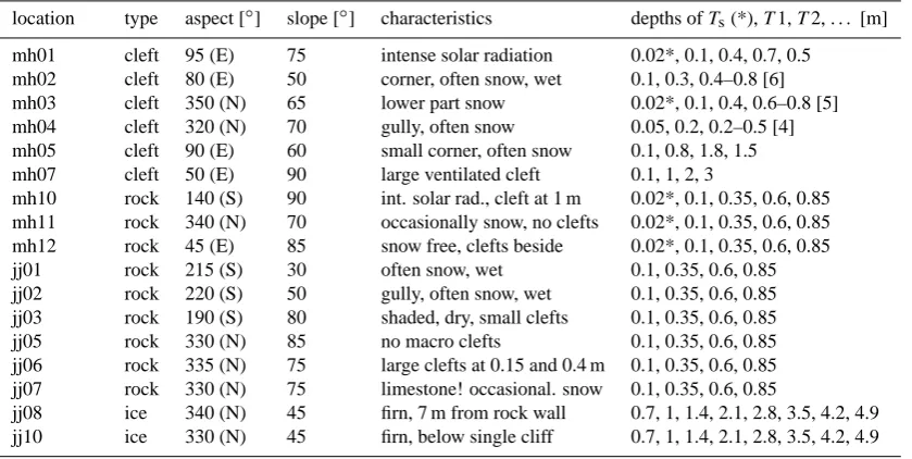
Table 1. Type and orientation of measurement locations with depth of the thermistors.
location type aspect [◦] slope [◦] characteristics depths ofTs(*),T1,T2, . . . [m]
mh01 cleft 95 (E) 75 intense solar radiation 0.02*, 0.1, 0.4, 0.7, 0.5 mh02 cleft 80 (E) 50 corner, often snow, wet 0.1, 0.3, 0.4–0.8 [6] mh03 cleft 350 (N) 65 lower part snow 0.02*, 0.1, 0.4, 0.6–0.8 [5] mh04 cleft 320 (N) 70 gully, often snow 0.05, 0.2, 0.2–0.5 [4] mh05 cleft 90 (E) 60 small corner, often snow 0.1, 0.8, 1.8, 1.5 mh07 cleft 50 (E) 90 large ventilated cleft 0.1, 1, 2, 3
mh10 rock 140 (S) 90 int. solar rad., cleft at 1 m 0.02*, 0.1, 0.35, 0.6, 0.85 mh11 rock 340 (N) 70 occasionally snow, no clefts 0.02*, 0.1, 0.35, 0.6, 0.85 mh12 rock 45 (E) 85 snow free, clefts beside 0.02*, 0.1, 0.35, 0.6, 0.85 jj01 rock 215 (S) 30 often snow, wet 0.1, 0.35, 0.6, 0.85 jj02 rock 220 (S) 50 gully, often snow, wet 0.1, 0.35, 0.6, 0.85 jj03 rock 190 (S) 80 shaded, dry, small clefts 0.1, 0.35, 0.6, 0.85 jj05 rock 330 (N) 85 no macro clefts 0.1, 0.35, 0.6, 0.85 jj06 rock 335 (N) 75 large clefts at 0.15 and 0.4 m 0.1, 0.35, 0.6, 0.85 jj07 rock 330 (N) 75 limestone! occasional. snow 0.1, 0.35, 0.6, 0.85
jj08 ice 340 (N) 45 firn, 7 m from rock wall 0.7, 1, 1.4, 2.1, 2.8, 3.5, 4.2, 4.9 jj10 ice 330 (N) 45 firn, below single cliff 0.7, 1, 1.4, 2.1, 2.8, 3.5, 4.2, 4.9
The aspect and slope indicated is the orientation of the surface 1–2 m around the sensor. The column characteristics contains remarks on special features such as the micro-topographic situation, snow cover, wetness and fracturation.
∗rock surface temperature (T
s) measured beside cleft or sensor rod.
[X] number in brackets indicate number of thermistors in the given depth range without exact depth information.
ice (about 0.05–0.3 m a−1), however, the distance between sensors remains constant. Based on the installation depth of 0.3 m and the evolution of the amplitudes of the uppermost sensor, we estimate its average depth during the measured period as 0.7 m from the surface (Table 1). The location of the surface temperature measurements are in similar local orientations at 0.1–1 m distance from the boreholes of the sensor rods or from the clefts.
The rock temperature measurements at Matterhorn aim to record the thermal conditions in snow-free and compact rock as a reference for the cleft temperature measurements and comparison to RST-measurements in other areas. Therefore, near-vertical bedrock of the three main aspects that persist at this field site (NW, NE, SE) was instrumented with sensor rods. For the locations mh10 and mh12, however, no suffi-ciently large compact rock mass could be found and clefts exist in proximity of the boreholes (Table 1). At Jungfrau-joch, the locations of the rock temperature measurements are selected to cover gradients in surface and near-surface condi-tions. For the two main aspects (N, S) different locations with respect to slope angle (snow retention), micro-topography (water availability; only at S) and fracturation where selected (Table 1). The two sensors that failed are the snow-covered one in the north face (jj09) and the sensor in unfractured rock at the south side (jj04). As a consequence, the effect of snow cover in the northern face and difference caused by fractura-tion for the south side could not be assessed at this field site.
3 Data processing
The raw data series contain invalid measurements or data gaps and the sampling interval of two minutes is slightly irregular. This demands a processing prior to the calcula-tion of the main parameters of interest. These are the mean annual temperatures (MATs) and temperature offsets (TOs) within the profiles (definition see below). First, invalid data is filtered and the remaining data is aggregated to regular in-tervals. After this, data gaps are filled. As these processing steps but also the characteristics and timing of the data acqui-sition introduce uncertainty into the computation of mean an-nual temperature an uncertainty analysis concludes this sec-tion.
3.1 Data validation, filtering and accuracy
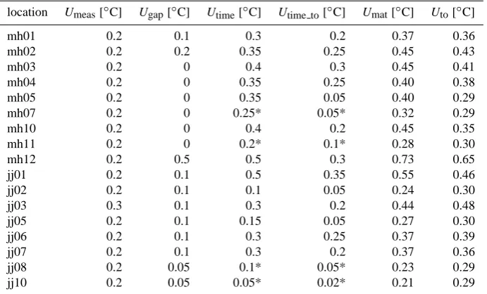
Table 2. Uncertainties of the MAT and the TO calculation.
location Umeas[◦C] Ugap[◦C] Utime[◦C] Utime to[◦C] Umat[◦C] Uto[◦C]
mh01 0.2 0.1 0.3 0.2 0.37 0.36 mh02 0.2 0.2 0.35 0.25 0.45 0.43
mh03 0.2 0 0.4 0.3 0.45 0.41
mh04 0.2 0 0.35 0.25 0.40 0.38 mh05 0.2 0 0.35 0.05 0.40 0.29 mh07 0.2 0 0.25* 0.05* 0.32 0.29
mh10 0.2 0 0.4 0.2 0.45 0.35
mh11 0.2 0 0.2* 0.1* 0.28 0.30 mh12 0.2 0.5 0.5 0.3 0.73 0.65 jj01 0.2 0.1 0.5 0.35 0.55 0.46 jj02 0.2 0.1 0.1 0.05 0.24 0.30 jj03 0.3 0.1 0.3 0.2 0.44 0.48 jj05 0.2 0.1 0.15 0.05 0.27 0.30 jj06 0.2 0.1 0.3 0.25 0.37 0.39 jj07 0.2 0.1 0.3 0.2 0.37 0.36 jj08 0.2 0.05 0.1* 0.05* 0.23 0.29 jj10 0.2 0.05 0.05* 0.02* 0.21 0.29
Umeas,UgapandUtime(Utime to) are the uncertainties introduced by the measurements, the gaps and the chosen time window.
Values indicate the confidence interval on a 95 % level.
∗
only data after July 2009 was considered for the estimation because of large bias by gaps prior to this date.
mh01). A second source of erroneous measurements is phys-ical damage of thermistors due to water entry or mechanphys-ical distortion. This type of invalid data cannot be easily filtered automatically because it is typically indicated by a slow drift of values that can best be detected by visual inspection and manual masking of the time span concerned. A similar man-ual masking of erroneous values was applied to the surface temperature measurements by individual thermistors because no reference values for this data exists.
The supplier of YSI 44006 thermistors guaranties an inter-changeability tolerance of±0.2◦C over a temperature range from –40◦C to +120◦C but tests in an ice-water bath showed that 95 % of the thermistors are within a range of±0.1◦C. A calibration of the assembled sensor could not be performed for logistic reasons, hence the accuracy of the installed sys-tem was not improved. Based on the stability of the reference resistors in the raw data we assume that the accuracy of a temperature measurement with the given setup including the effect of aggregation is±0.2◦C for all sensors except jj03 with±0.3◦C (Table 2).
3.2 Gap filling algorithm and mean annual temperature (MAT) calculation
Running arithmetic averages over 365 days are calculated and result in a continuous time-series of MAT values. These time-series are used to evaluate the uncertainty of the MAT value for one particular time window: in general the MAT presented is for the hydrological year 2010 (see below). Missing data within the considered time window affects the
Fig. 6. Example of gap-filling with original values (red) and the
resulting dataset after gap filling (blue). Note that the data in this graph (mh01;T1)is a worst case concerning gap frequency.
was evaluated by introducing the same gaps into the com-plete time series; this showed that an approximation of the true MAT to better than±0.1◦C was achieved with gap fill-ing compared to±1◦C if gaps contain no values. Sensors mh02 and mh12 contain larger gaps and therefore introduce a larger uncertainty into the MAT estimate (Table 2). 3.3 Definition and calculation of the temperature offset
(TO)
For practical reasons we use the measured offset between the MAT at top and bottom of the profiles and call them
tem-perature offset (TO). This parameter deviates from the ther-mal offset defined as the difference between the temperature
below the active layer at the permafrost table (TTOP) and the MAGST (Burn and Smith, 1988). In fractured bedrock a quantification of the thermal offset is impractical, because of: (a) highly variable MAGST; (b) highly variable active layer thickness. The thermal offset is expected to be larger than our empirical TO in some cases. However, the values for offsets and MAT variability given in this study have an exemplary character and indicate possible ranges because many degrees of freedom exist in the possible variations of controlling pa-rameters.
To quantify the temperature difference between the near-surface and greater depth, the MAT ofT4 is subtracted from the one ofT1 or for the ice face,T8 fromT1. Hence, pos-itive differences indicate a higher MATs with depth while negative TO-values appear in situations where the subsurface is colder than the surface. As the MATs are continuous time-series (running annual mean), the TO may be calculated for every day as well (cf. Fig. 7). The rock surface temperature measurements (Ts) are not considered for this calculation to avoid a mix of rock and cleft temperatures and to keep sen-sor rod measurements with and without Ts comparable. For mh02T6 is taken instead ofT4 because the MAT of the latter one is missing.
3.4 Uncertainty analysis of mean annual temperatures and temperature offsets
Three main sources of uncertainty (Table 2) affect our esti-mate of the MAT: (a) systematic measurement errors (Umeas), (b) data gaps (Ugap), and (c) the period for which the mean is calculated (Utime,Utime to).Umeasis given by the measure-ment accuracy (Sect. 3.1) because the bias from the mea-surement is systematic over the whole time series and is not significantly reduced by the averaging. ForUgapthe values are estimated dependent on quantity of missing data in the averaging window (Sect. 3.1) but lower values are chosen in case of the ice temperatures due to smooth time series and correspondingly better performance of the gap-filling algo-rithm. MAT calculations are influenced by the start and end date of the averaging window on the long term (inter-annual variation of MAT) but also on the short term (seasonal) if
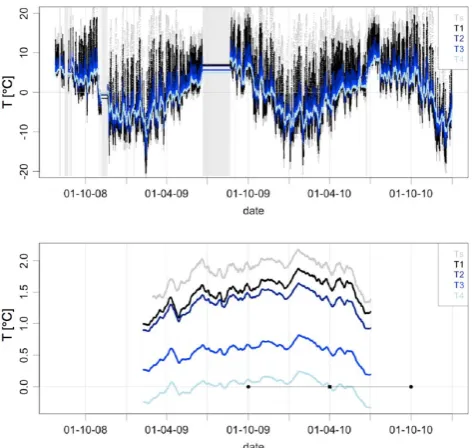
Fig. 7. Time series from July 2008 to the end of 2010 of the rock
temperature measurements (top) at mh10 with interpolated values in data gaps (grey bars) and corresponding running annual means (bottom) that are represented in the center of the averaging window. The black dots indicate this averaging window for one MAT with the quad showing the point in time of its representation. For most sensors this averaging window was chosen to minimize data gaps.
the temperature time series show strong weekly variations. Figure 7 shows the temperature time series and the seasonal variation of the MAT for the sensor rod at mh10 (rock). This variation is considered as uncertaintyUtime for the compar-ison of the MATs because it is not correlated between loca-tions. The MAT values for all sensors except jj01, mh04 and mh12 are calculated for 1 October 2009 to 1 October 2010 (Fig. 7 black dots). The variation of the MAT is, however, in-fluenced by data gaps, hence for three sensors the part of the time series with large gaps is excluded from the estimation of Utimethat is performed by the difference of 2.5 and 97.5 % quantiles (Table 2). As the running annual means of the tem-peratures at different depth but at the same location are cor-related (Fig. 7), the temperature offset (TO) varies less over time. For that reasonUtime to is estimated as a measure of the uncertainty in temperature offset calculation, introduced by timing of the averaging interval, which is in most cases smaller thanUtime(Table 2).
The total uncertainties of the MAT (Umat)and the TO (Uto) are calculated by quadratic addition of the uncertainties ac-cording to the addition of spreads:
Umat=
q U2
meas+Ugap2 +Utime2 (1)
Uto=
q 2·U2
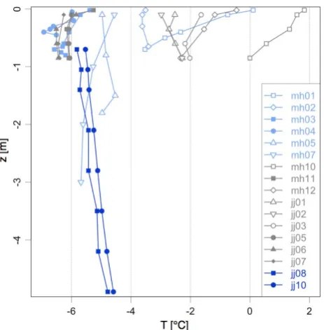
Fig. 8. Mean annual temperature (MAT) profiles for clefts (light
blue), rock (grey) and ice (dark blue) with depth z measured perpen-dicular to the surface. Solid symbols are shaded locations (north); hollow symbols are more exposed to solar radiation (south and east). Note that the uppermost MAT of mh01 to mh03 is a rock surface temperature (Table 1).
Contrary to Eq. (1), theUmeasterm is multiplied by a fac-tor of two in Eq. (2) because the independent uncertainties of two temperature measurements contribute toUto. Ugap of two measurements in the same profile are correlated and therefore their single consideration is a worst case. However this influence is negligible in most cases anyway (Table 2). The resulting uncertainties that are relevant for the interpre-tation of the MAT and the TO are listed in Table 2. These un-certainties are used in the following to evaluate if the MATs are significantly different and if significant TOs exists.
4 Results
4.1 Mean annual temperatures (MATs)
Figure 8 gives an overview of the MATs of the clefts, rock and ice ordered by location and type (colors). The repre-sentation as profiles with z being the distance from surface does not show the real distance between the sensors and lat-eral offsets in the thermistor position are masked in case of the cleft and ice temperatures. The MAT values from the north-oriented locations cluster around –6◦C (Fig. 8) and are slightly warmer (0.5–1.5◦C) than the MAAT (–6.7 to –7.3◦C). Remarkable is the exact match in mean annual rock/ground temperature (MAGT) of mh11 and jj05, which are both in intact steep rock (Fig. 8; for a better
differentia-tion of these values see also Fig. 8). The mean temperatures at the surface (MAGST) at the more sun-exposed locations are 1–8◦C higher than the shaded ones and the same is true for the near-surface cleft temperatures (MAT ofT1)(Fig. 8). The difference in MAGT between sunny and shaded loca-tions is more pronounced at Matterhorn than at Jungfrau-joch. This is because the south face MAGT at Matterhorn (mh10) is 3–4◦C higher forT1 (0.1 m) and 2◦C higher for T4 (0.85 m) than the ones at Jungfraujoch (jj01, jj02 and jj03) (Fig. 8).
Cleft MATs of the east-oriented locations at Matterhorn are significantly lower than the MAGT at locations with com-parable orientation: the cleft at mh07 is 4◦C colder at the top and 3◦C colder at depth than the rock at mh12 which is only a few meters above in the same face; the two clefts mh02 and mh05 are 2–3◦C colder than mh12 although they face more toward south; at depth, even the radiation-exposed pro-file mh01 is colder than mh12 (Fig. 8). The MAT-propro-files from the ice faces start around –5.5◦C near the surface and show a constant positive temperature gradient with depth of approximately +0.2◦C m−1(Fig. 8). The near-surface MAT in the ice is 0.2–0.8◦C higher than in the rock face just above the ice face, hence the difference found is marginal.
4.2 Temperature offsets (TOs)
Figure 8 shows the temperature offsets (TOs) from Matter-horn and Jungfraujoch. The difference in depth between the two thermistors that are used for the TO calculation is only constant for the rock temperatures (cf. Fig. 8), hence, the TO-values in Fig. 9 are directly comparable for the rock measure-ments but smaller or larger depth ranges need to be consid-ered for the cleft and ice temperatures.
In total, seven TOs are negative, four are positive and six lie within the uncertainty range (Fig. 9). More than half (4) of the clearly negative TOs are detected within the clefts, the two most positive TOs consist of the ice face mea-surements. The locations with highest surface temperatures (mh01, mh10 and mh12) have most negative TOs and are all located at Matterhorn (2 in rock, 1 in cleft). From the rock temperatures at Jungfraujoch, only one sensor shows nega-tive and one posinega-tive TO, whereas all the other sensors have no significant TO. This is in contrast to the Matterhorn data where seven out of nine cleft and rock sensors show a sig-nificant TO (Fig. 9). A further regularity is, that all sensors with a slight or significant positive TO are located relatively flat and accumulate often a snow cover (cf. Table 1). 4.3 Seasonal temperature variation and inter-annual
variability of MAT
Fig. 9. Mean annual temperature (MAT) and temperature offset
(TO) between cleft top and within cleft (light blue); in shallow rock boreholes (grey) and in ice (dark blue). The black error bars show the uncertaintiesUtoof the temperature offset estimates on a 95 %
confidence level. The letters at the top indicate the main aspect of the locations (E = east, N = north, S = south). The location labels given in the middle of the figure help to read other attributes from Table 1. At the bottom, the location type is denoted, which corre-sponds to the colours of the bars from the thermal offset.
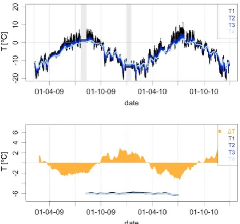
examples. The data from jj05 serves as a reference for a rock temperature profile that has no significant TO (Fig. 10): the 30-days running mean of1T has similar negative and positive amplitudes (±2◦C) and results in a TO close to zero if averaged over a year. This is also shown with the overlapping MATs that at the same time indicates the small seasonal variation (compare with Utime in Table 2). In Figs. 11 and 12 two examples of time series are presented to illustrate, which periods of the year are responsible for the temperature offsets and what explains large variations of the MATs and TOs between different years: the time series of the cleft mh01 shows large seasonal variations and very large daily amplitudes in spring and summer that are not symmet-rical with the temperatures at depth and cause a negative1T from March to November for both years (Fig. 11). Similar seasonal patterns are found at all sensors with large negative TOs (mh07, mh10, mh12). In contrast, at jj01 (rock) positive temperatures and large daily amplitudes atT1 are limited to the snow free period in summer and the winter temperatures
Fig. 10. Time series of rock temperatures at jj05 (TO = 0◦C) mea-sured every 10’ (top) and the temperature difference1T =T4−T1 averaged over 30 days (bottom). Additionally the running MATs are ploted in lines similar to Fig. 7 (bottom). Jj05 is a sensor rod at a shadowy location.
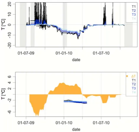
are smoothed by the snow cover (Fig. 12). Because the snow-free periods differ between 2009 and 2010 and the tempera-tures at depth are buffered by thawing ground ice (zero cur-tains), the summer1T varies strongly and the TO changes from positive to negative values (Fig. 12).
5 Discussion
5.1 Surface characteristics and temperature variability
Recent studies on the small-scale variability of mean annual ground surface temperatures (MAGST) in gentle mountain slopes, found a variability of 0.16–2.5◦C within 10 m×10 m footprints (Gubler et al., 2011) and 1.5–3.0◦C over distances of 30 to 100 m (Isaksen et al., 2011). With the rough micro-topography typical for steep fractured bedrock, we expect MAGST-variabilities at the upper end of this range.
Fig. 11. Time series of mh01 with measured temperatures (top) and
the temperature difference1T averaged over 30 days as well as
MATs (bottom). Mh01 is a cleft at a location with intense irradia-tion.
Fig. 12. Time series of jj01 with measured temperatures (top) and
the temperature difference1T averaged over 30 days as well as
MATs (bottom). Jj01 is a sensor rod at a location that accumulates snow.
more convective cloudiness in the afternoon and the climatic situation (orographic clouds at the northern divide). The data from the defect sensor jj04 (T3 andT4 have sufficient data to calculate annual means), however suggests that MAGT in the range of –0.5◦C occur at the south slope of
Jungfrau-joch as well. Hence, we assume other factors such as snow retention (jj01, jj02), cooling by melt water (jj02) and local shading (jj03, jj02) due to the micro-topographic situation as mainly responsible for the lower near-surface MAGTs at the Jungfraujoch south face (Table 1; Fig. 4). The same cool-ing effect by local snow cover and more shadcool-ing due to the concave micro-topography may be responsible for the lower cleft MATs at mh02 and mh05 in comparison with the near-surface MAT of mh01 that has the same orientation. This net cooling effect of the snow cover is in contrast to the net warming effect on more gentle slopes where thick snow cover cause a preponderance of “warming” by winter insula-tion over the “cooling” by increased albedo, emissivity and latent heat consumption (Keller and Gubler, 1993). In steep slopes at high elevation the thinner snow cover and summer snowfalls could result in a reverse effect (Pogliotti, 2011). This is supported by the data from jj01 showing that the sur-face remains snow-covered in the period with most intense solar irradiation (June and July) and that winter cooling indi-cated by upward heat fluxes (1T = +4◦C; larger than e.g. at jj05) is not prevented (Fig. 12).
5.2 Non-conductive processes and near-surface temperature offsets
The variation of mean annual ground temperatures within the active layer is usually described with the thermal offset (see Sect. 3.3). This effect is well-known in arctic soils, and Gru-ber and HaeGru-berli (2007) proposed three possible sources of thermal offsets making its importance also likely in steep fractured bedrock: (1) variable thermal conductivity due to saturation and phase changes of pore water (thermal diode effect of rock); (2) changes of the heat transport across clefts as a consequence of freeze/thaw/runoff of cleft ice (thermal diode effect of clefts); (3) ventilation effects within loose block cover on less steep parts of rock faces. All these pro-cesses are expected to reduce temperatures at depth com-pared with MAGST and hence lead to lower TO-values in our measurements.
The negative TO of 0.5–1.5◦C measured in rock (mh10, mh12, jj06) is well explained by the cooling within the clefts because all three boreholes are in proximity to open clefts (Table 1). Changes in thermal conductivity due to phase change of cleft and pore water (in case of jj06 the borehole crosses two clefts) could be an additional source of a negative TO at mh03 and mh06 (Gruber and Haeberli, 2007; Pogliotti et al., 2008). The seasonal pattern of1T (Sect. 4.3) fits best
to the ventilation hypothesis for clefts because: (a) the out-ward heat flux in winter would reduce1T (all sensors); (b)
radiation can not directly affect the upper most thermistor T1 of the sensors mh01 (snow) and mh07 (shading) in win-ter; (c) ventilation in winter is reduced due to snow in clefts (mh01, mh03, mh04). The other processes that are related to phase changes are more likely to produce a 1T pattern
that corresponds to freeze-thaw transitions. Slightly or sig-nificantly positive TOs occur all at comparably flat locations that are often snow-covered (Table 1). The described reduc-tion of the local near-surface temperature and possibly the influence of sensible heat release at depth by percolating wa-ter (Hasler et al., 2011) explain the positive TOs except for the offset at jj02 where most likely small-scale 3-D effect cause higher MAGTs at depth: a radiation exposed surface that is less snow covered is 0.8 from the drilling location and affects the measured temperature profile laterally (Fig. 4). 5.3 Thermal regime in ice faces
In the ice face, near-surface temperatures do not significantly differ from the rock face above, hence the different albedo from the rock and ice (firn) surface has a minor effect at this shaded face. In contrast to the rock, however, the temper-ature gradient with depth is +0.23◦C m−1 and results in a positive TO between 0.7 m and 5 m depth. Possible sources of such positive TOs are (a) stationary upward directed heat fluxes; (b) transient effects of a surface cooling; (c) lateral effects of the non-perpendicular drilling; (d) advection of sensible heat by ice/firn motion (Luethi and Funk, 2001); (e) latent heat release by percolation and refreezing water (Hoelzle et al., 2011). We exclude (b), (c) and (d) as ex-planation for the observed offset because of the linear tem-perature profiles (Fig. 8), no evidence for a surface cooling, the small lateral variability and the low ice flow velocity due to the proximity to the upper end of the ice face. In the present data we cannot identify a depth of maximal la-tent heat release (bent temperature profile), which should be typical for process (e) (Fig. 8). It is unclear whether this depth of heat release may be below the profile causing an upward heat flux, because little is known about the inter-nal structure and permeability of such ice faces. Geothermal heat fluxes and 3-D effects within the Sphinx ridge (Weg-mann, 1998; Noetzli et al., 2007) driven by the warm south side and the infrastructure are more likely to explain the ob-served temperature profiles. Assumptions for the geothermal heat flux (ht<0.03 W m−2)and conductivity of porous ice
(λ >1.5 W m−1K−1)result in a significantly smaller temper-ature gradient (dT /dz <0.02◦C m−1). The lateral heat flux may be, however, ten times larger (ht = 0.3 W m−2)due to the warm southern side and the heat introduced by the infrastruc-ture within the ridge (Wegmann, 1998) induce a temperainfrastruc-ture gradient within the ice face in the order of 0.2◦C m−1.
6 Conclusions and perspectives
The thermal conditions of steep bedrock permafrost and ice faces where studied based on 17 shallow temperature pro-files. On the basis of two-year time series from two field sites in the Swiss Alps, we calculated the mean annual tem-peratures (MAT) and their temperature offsets (TO) within the profiles and analyzed them with respect to their micro-topographic situation, surface and near-surface characteris-tics. The main findings are:
– Differences in MAT and TO are highly significant with respect to the uncertainty introduced by measurement errors, data gaps and temporal variations.
– When using MAGST as an indication for the permafrost temperature in mountain faces, one needs to account for temperature offset, similar to the thermal offset in arctic lowland areas.
– The ice face investigated in this study has similar MAT as the rock beside and no clear evidence for TO by latent heat release from percolation effects was found. – Snow cover likely reduces MAGST (2–3◦C) of
mod-erately steep (45–70◦) locations in radiation-exposed faces at high elevation because it often persists for the period with most intense radiation (June).
– A ventilation effect of clefts causes negative TO and lower temperatures at depth (≈1.5◦C) for strongly frac-tured near-vertical bedrock at radiation-exposed loca-tions.
– Other processes such as thermal diode effects and lo-cal shading may support colder MAT but could not be quantified with the available data.
– Local warming within clefts by heat advection of per-colating water shows minor effects on MAT, however, it should be considered in respect of rock stability. – Summarizing the previous statements we postulate that
radiation-exposed steep rock faces with intermitted snow patches and/or large fractures are up to 3◦C lower at depth than expected from MAGST at snow-free loca-tions.
which may in fact extend to lower elevations by several hun-dred meters in radiation-exposed faces than expected so far. Corresponding effects could be parameterized by the use of surface and near-surface characteristics that affect snow re-tention and ventilation. For an application and extrapola-tion of these findings the following may be reflected: (a) the two effects should be considered to be complementary rather than cumulative, because snow reduces the efficiency of the ventilation; (b) the ventilation effect depends on cleft aper-ture and frequency, hence near-surface characteristics need to provide information on this aspect; and (c) the effect of snow cover could change with elevation due to a changed duration of the snow-free period. To estimate the latter, the near-surface temperature profiles may be used to calibrate the snow cover in a physically oriented permafrost models for steep bedrock: the measured gradients in the near-surface layer can serve as a direct estimate of the heat flux through the snow cover. As long as no further analysis and model-based spatial extrapolation of these findings is performed, we suggest to include up to 3◦C lower temperatures in radiation-exposed rock faces in the uncertainty indications of MAGT estimates.
Acknowledgements. We would like to thank the PermaSense team,
J. Beutel, R. Lim, M. Y¨ucel, I. Talzi, T. Gsell, M. Keller, L. Thiele and C. Tschudin, who made these challenging measurements possible. The presented research was funded within the project PermaSense by the Swiss Federal Office for the Environment (FOEN) and the Swiss National Foundation (SNF) NCCR-MICS. The fieldwork at Jungfraujoch was supported by the International Foundation High Altitude Research Stations Jungfraujoch and Gornergrat (HFSJG) and benefited from the friendly support of the Jungfrau Railways and their staff.
Edited by: M. Stendel
References
Allen, S. K., Gruber, S., and Owens, I. F.: Exploring steep bedrock permafrost and its relationship with recent slope failures in the Southern Alps of New Zealand, Permafrost Periglac., 20, 345– 356, 2009.
Beniston, M.: Mountain climates and climatic change: An overview of processes focusing on the European Alps, Pure Appl. Geo-phys., 162, 1587–1606, 2005.
Beutel, J., Gruber, S., Hasler, A., Lim, R., Meier, A., Plessl, C., Talzi, I., Thiele, L., Tschudin, C., Woehrle, M., and Yuecel, M.: PermaDAQ: A scientific instrument for precision sensing and data recovery in environmental extremes, Proceedings of the 2009 International Conference on Information Processing in Sensor Networks, IEEE Computer Society, 265–276, 2009. Burn, C. R. and Smith, C. A. S.: Observations of the “thermal
off-set” in near-surface mean annual ground temperatures at sev- eral sites near Mayo, Yukon Territory, Canada, Arctic, 41, 99–104, 1988.
Coutard, J. P. and Francou, B.: Rock temperature measurements in two alpine environments: implications for frost shattering, Arctic Alpine Res., 21, 399–416, 1989.
Gruber, S. and Haeberli, W.: Permafrost in steep bedrock slopes and its temperature-related destabilization following climate change, J. Geophys. Res., 112, F02S18, doi:10.1029/2006JF000547, 2007.
Gruber, S., Hoelzle, M., and Haeberli, W.: Rock-wall temperatures in the Alps: modelling their topographic distribution and regional differences, Permafrost Periglac., 15, 299–307, 2004.
Gubler, S., Fiddes, J., Keller, M., and Gruber, S.: Scale-dependent measurement and analysis of ground surface temper-ature variability in alpine terrain, The Cryosphere, 5, 431–443, doi:10.5194/tc-5-431-2011, 2011.
Haeberli, W., Wegmann, M., and Vonder Muehll, D.: Slope stability problems related to glacier shrinkage and permafrost degradation in the Alps, Ecologae Geologicae Helveticae, 90, 407–414, 1997. Hanson, S. and Hoelzle, M.: The thermal regime of the active layer at the Murtel rock glacier based on data from 2002, Permafrost Periglac., 15, 273–282, 2004.
Harris, S. A. and Pedersen, D. E.: Thermal regimes beneath coarse blocky materials, Permafrost Periglac., 9, 107–120, 1998. Hasler, A., Gruber, S., Font, M., and Dubois, A.: Advective heat
transport in frozen rock clefts - conceptual model, laboratory ex-periments and numerical simulation, Permafrost Periglac. Pro-cess., accepted, 2011.
Hasler, A., Talzi, I., Beutel, J., Tschudin, C., and Gruber, S.: Wireless sensor networks in permafrost research: concept, re-quirements, implementation, and challenges, in: Proceeding of the Ninth International Conference on Permafrost, Fairbanks, Alaska, USA, 669–674, 2008.
Hiebl, J., Auer, I., B¨ohm, R., Sch¨oner, W., Maugeri, M., Lentini, G., Spinoni, J., Brunetti, M., Nanni, T., and Perec, Tadi, M.: A high-resolution 1961–1990 monthly temperature climatology for the greater Alpine region, Meteorol. Z., 18, 507–530, 2009. Hoelzle, M., Darms, G., L¨uthi, M. P., and Suter, S.: Evidence of
accelerated englacial warming in the Monte Rosa area, Switzer-land/Italy, The Cryosphere, 5, 231–243, doi:10.5194/tc-5-231-2011, 2011.
Isaksen, K., Oedegard, R. S., Etzelmueller, B., Hilbich, C., Hauck, C., Farbrot, E., Hygen, H. O., and Hipp, T. F.: Degrading moun-tain permafrost in southern Norway: spatial and temporal vari-ability of mean ground temperatures, 1999–2009, Permafrost Periglac., doi:10.1002/ppp.728, in press, 2011.
Keller, F. and Gubler, H.: Interaction between snow cover and high mountain permafrost, Murtel-Corvatsch, Swiss Alps, in: Pro-ceedings of the Sixth International Conference on Permafrost, 332–337, 1993.
Luethi, M. P. and Funk, M.: Modelling heat flow in a cold, high-altitude glacier: interpretation of measurements from Colle Gnifetti, Swiss Alps. J. Glaciol., 47, 314–324, 2001.
Matsuoka, N.: Frost weathering and rockwall erosion in the south-eastern Swiss Alps: Long-term (1994–2006) observations, Geo-morphology, 99, 353–368, 2008.
Matsuoka, N. and Sakai, H.: Rockfall activity from an alpine cliff during thawing periods, Geomorphology, 28, 309–328, 1999. Noetzli, J., Gruber, S., Kohl, T., Salzmann, N., and Haeberli, W.:
Res, 112, F02S13, doi:10.1029/2006JF000545, 2007.
Noetzli, J., Gruber, S., and Poschinger, A.: Modellierung und Mes-sung von Permafrosttemperaturen im Gipfelgrat der Zugspitze, Deutschland, Geographica Helvetica, 65, 2, 113–123, 2010. PERMOS: Permafrost in Switzerland 2006/2007 and 2007/2008, in:
Glaciological Report (Permafrost) No. 8/9 of the Cryospheric Commission of the Swiss Academy of Sciences, edited by: Noetzli, J. and Vonder Muehll, D., 2010.
Pogliotti, P.: Influence of Snow Cover on MAGST over Com-plex Morphologies in Mountain Permafrost Regions, PhD The-sis, Turin, Italy, Universit`a degli Studio di Torino, 2011.
Pogliotti, P., Cremonese, E., Morra di Cella, U., Gruber, S., and Gi-ardino, M.: Thermal diffusivity variability in alpine permafrost rock walls, In Proceeding of the Ninth International Conference on Permafrost, Fairbanks, Alaska, USA, 1427–1432, 2008. Wegmann, M.: Frostdynamik in hochalpinen Felsw¨anden am
Beispiel der Region Jungfraujoch – Aletsch, Mitteilungen der Versuchsanstalt f¨ur Wasserbau, Hydrologie und Glaziologie der ETH Z¨urich, 161, 1998.