M E T H O D O L O G Y
Open Access
Prediction of donor splice sites using
random forest with a new sequence
encoding approach
Prabina Kumar Meher
1†, Tanmaya Kumar Sahu
2†and Atmakuri Ramakrishna Rao
2** Correspondence:rao.cshl.work@ gmail.com
†Equal contributors 2
Centre for Agricultural Bioinformatics, Indian Agricultural Statistics Research Institute, New Delhi 110 012, India
Full list of author information is available at the end of the article
Abstract
Background:Detection of splice sites plays a key role for predicting the gene structure and thus development of efficient analytical methods for splice site prediction is vital. This paper presents a novel sequence encoding approach based on the adjacent di-nucleotide dependencies in which the donor splice site motifs are encoded into numeric vectors. The encoded vectors are then used as input in Random Forest (RF), Support Vector Machines (SVM) and Artificial Neural Network (ANN), Bagging, Boosting, Logistic regression,kNN and Naïve Bayes classifiers for prediction of donor splice sites.
Results:The performance of the proposed approach is evaluated on the donor splice site sequence data ofHomo sapiens, collected from Homo Sapiens Splice Sites Dataset (HS3D). The results showed that RF outperformed all the considered classifiers. Besides, RF achieved higher prediction accuracy than the existing methods viz., MEM, MDD, WMM, MM1, NNSplice and SpliceView, while compared using an independent test dataset.
Conclusion:Based on the proposed approach, we have developed an online prediction server (MaLDoSS) to help the biological community in predicting the donor splice sites. The server is made freely available at http://cabgrid.res.in:8080/ maldoss. Due to computational feasibility and high prediction accuracy, the proposed approach is believed to help in predicting the eukaryotic gene structure.
Keywords:Di-nucleotide association, Machine learning, PWM, Computational feasibility
Background
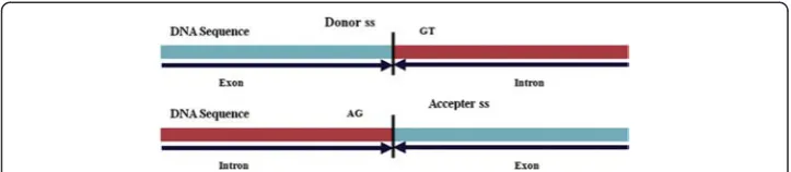
Prediction of gene structures is one of the important tasks in genome sequencing pro-jects, and the prediction of exon-intron boundaries or splice sites (ss) is crucial for pre-dicting the structures of genes in eukaryotes. It has been established that accurate prediction of eukaryotic gene structure highly depends upon the ability to accurately identify the ss. The ss at the exon-intron boundaries are called the donor (5′) ss whereas intron-exon boundaries are called the acceptor (3′)ss. The donor and acceptor sswith consensus GT (at intron-start) and AG (at intron-end) respectively are known as canonicalss (GT-AG type; Fig. 1). Approximately, 99 % of thess are canonical GT-AG typess[1]. As GT-and AG-are conserved in donor and acceptorssrespectively, every GT
and AG in a DNA sequence could be a donor or acceptor ss. However, they need to be predicted as either real (true) or pseudo (false)ss.
During the last decade, several computational methods have been developed for ss detection that can be grouped into several categories viz., probabilistic approaches [2], ANNs [3, 4], SVM [5–7] and information theory [8]. These methods seek the consen-sus patterns and identify the underlying relationships among nucleotides in ss region. ANNs and SVMs learn the complex features of neighborhood nucleotides surrounding the consensus di-nucleotides GT/AG by a complex non-linear transformation, whereas the probabilistic models estimate the position specific probabilities of ss by computing the likelihood of candidate signal sequences. Roca et al. [9] identified the di-nucleotide dependencies as one of the main features of donor ss. Although the above mentioned methods are complex and computationally intensive, it is evident that position specific signals and nucleotide dependencies are pivotal forssprediction.
In the class of ensemble classifiers, RF [10] is considered as highly successful one that consists of ensemble of several tree classifiers (Fig. 2). The wide application of RF for prediction purposes in biology can be seen from literature. Hamby and Hirst [11] utilized the RF algorithm for prediction of glycosylation sites and found significant increase in accuracy for the prediction of“Thr”and“Asn”glycosylation sites. Jain et al. [12] assessed the performance of different classifiers (fifteen classifiers from five differ-ent categories of pattern recognition algorithms) while trying to solve the protein
Fig. 1Pictorial representation of donor and acceptorss. Donorsshave di-nucleotides GT at the beginning of the intron and acceptorsshave di-nucleotides AG at the end of intron
folding problem. Their experimental results showed that RF achieved better accuracy as compared to the other classifiers. Later on, Dehzangi et al. [13] demonstrated that the RF classifier enhanced the prediction accuracy as well as reduced the time con-sumption in predicting the protein folds. In the recent past, Khalilia et al. [14] used RF to predict disease risk for eight disease categories and found that the RF outperformed SVM, Bagging and Boosting.
Keeping the above in view, an attempt has been made to develop a computational approach for donorssprediction. The proposed approach involves sequence encoding procedures and application of RF methodology. For given encoding procedures, RF outperformed SVM, ANN in terms of prediction accuracy. Also, RF achieved higher accuracy while compared with existing approaches by using an independent test dataset.
Methods
Collection and processing of splice site data
The true and false ss sequences of Homo sapiens were collected from HS3D [15] (http://www.sci.unisannio.it/docenti/rampone/). The downloaded dataset contains a total of 2796 True donor Splice Sites (TSS) (http://www.sci.unisannio.it/docenti/ram-pone/EI_true.zip) and 90924 False donor Splice Site (FSS) (http://www.sci.unisannio.it/ docenti/rampone/EI_false_1.zip). The sequences are of 140 bp long with conserved GT at 71stand 72ndpositions respectively.
Both introns and exons have important role in the process of pre-mRNA splicing. To be more specific, presence of conserved-ness at both 5′and 3′ends of intron as well as exonic splicing enhancers [16, 17] is vital from splicing point of view. Besides, the length of an exon is also an important property for proper splicing [18]. It has been shown in vivo that internal deletion of consecutively recognized internal exons that are below ~50 bp may often lead to exon skipping [19]. As far as the length of an intron is concerned, Zhu et al. [20] carried out the functional analysis of minimal introns ranging between 50-100 bp and found that minimal introns are conserved in terms of both length and sequence. Hence, the window length of 102 bp [50 bp at exon-end + (GT + 50 bp) at intron-start] is considered here (Fig. 3).
Though in longer window length there is a less chance of existence of identical se-quences, still we performed redundancy check to remove the identical TSS sequences from the dataset. To train the model efficiently, same number of unique FSS (equal to unique TSS) was considered by drawing at random from 90924 FSS. A sequence similarity search was then performed to analyze the sequence distribution, where each sequences of TSS was compared with the remaining sequences of TSS as well as with all the sequences of FSS and vice versa. The percentage of similarity between any two sequences was
Fig. 3Pictorial representation ofssmotif. The di-nucleotides GT conserved at 51stand 52ndpositions in the
computed by assigning a score of 1 and 0 for every match and mismatch in nucleotides respectively, and the same is explained below for two sample sequences.
Sequence 1: ATTCGTCATG Sequence 2: TCTAGTTACG Score : 0010110101
Similarity (%)=(5/10)*100=50
Further, we prepared a highly imbalanced dataset consisting of 5%TSS and 95%FSS to assess the performance of RF as well as to compare its performance with that of SVM and ANN.
Computation of Position Weight Matrix (PWM)
The sequences of both TSS as well as FSS were position-wise aligned separately, using the di-nucleotide GT as the anchor. This position-wise aligned sequence data was then used to compute the frequencies and probabilities of nucleotides at each position. From a given set S of Naligned sequences each of length l,s1,…,sN, where sk=sk1,…, skl (skj є{A, C, G, T},j= 1, 2,…,l), the PWM was computed as
pij¼
1 n
Xn
k¼1 Ii skj
i¼A;C;G;T
j¼1;2;…;l
where Iið Þ ¼q
1if i¼q
0otherwise 8
< : 8
<
: ð1Þ
The PWM with four rows (one for each A, C, G, and T) and 102 columns i.e., equal to the length of the sequence (Fig. 4) was then used for computing the di-nucleotide as-sociation scores.
Di-nucleotide association score
The adjacent di-nucleotide association scores are computed under proposed encoding procedures as follows:
1. In thefirstprocedure (P-1), the association between any two nucleotides occurring at two adjacent positions was computed as the ratio of the observed frequency to the frequency due to random occurrence of the di-nucleotide. ForNposition-wise aligned sequences, numerator is the number of observed di-nucleotide occurring together, whereas the denominator isNtimes of 0.0625 (=1/16, probability of occurrence of any di-nucleotide at random).
2. In thesecondprocedure (P-2), the association was computed as the ratio of the observed frequency to the expected frequency, where expected frequency was computed from PWM under the assumption of independence between the positions.
3. In thethirdprocedure (P-3), the di-nucleotide association was computed as the ab-solute value of the relative deviation of the observed frequency from the expected frequency, where expected frequency was computed as outlined in P-2.
In all the three procedures, the scores were transformed to logarithm scale (base 2) to make them uniform. The computation of the di-nucleotide association scores is ex-plained as follows:
Letpjibe the probability of occurrence ofithnucleotide atjthposition,pi′
j′ be the
prob-ability of occurrence ofi′thnucleotide atj′thposition andnij;;ij′′ be the frequency of
oc-currence of ith and i′th nucleotides together atjth and j′th positions respectively. Then the different di-nucleotide association scores betweenith andi′thnucleotides occurring atjthandj′thpositions under P-1, P-2, P-3 were computed using following formula
P−1
ð Þ→sð Þi;i′
j;j′
ð Þ ¼ log2
nij;;ij′′ N0:0625 0
@
1 A
P−2
ð Þ→sð Þi;i′
j;j′
ð Þ ¼ log2
nij;;ij′′ Npi
jpi
′ j′ 0 @ 1 Aand
P−3
ð Þ→sð Þi;i′
j;j′
ð Þ ¼ log2
nij;;ij′′−Npijpi
′
j′
Npi
jpi
′ j′
ð2Þ
respectively, where sð Þi;i′
j;j′
ð Þ is the association score, Nis the total number of sequence motifs in the data set; i,i′є{A,T, G, C} andj= 1, 2,…, (window length-1) and j′=j+ 1. A pseudo count of 0.001 was added to avoid the logarithm of zero in the frequency. For a clear understanding, computation of di-nucleotide association scores is given below, through an example with 5 different sequences.
Positions : 0123456789 Sequence 1: ATACGTCATG Sequence 2: TGTAGTTTCG Sequence 3: ATGCGTACAC Sequence 4: GACTGTTGCT Sequence 5: CCTGGTGAGA
Using these sequences, the random, observed and expected (under independence) frequencies for di-nucleotide AT occurring at positions 0, 1 respectively are computed as follows:
Observed frequency = Number of times AT occurs together at 0thand 1st positions respectively
Random frequency = Number of sequences × Probability of occurrence of any of the 16 combinations of di-nucleotides at random (=1/16)
=5*0.0625 =0.3125
Expected frequency under independence = Number of sequences × Probability of in-dependent occurrence of A at 0thposition × Probability of independent occurrence of T at 1stposition
=5*(2/5)*(2/5) =0.8
In similar way, the frequencies can be calculated for other possible di-nucleotide combinations (AA, AG, AC, TA, …, CC) occurring at all possible adjacent positions. Now, the association scores for three different procedures P-1, P-2 and P-3 can be cal-culated by using equation (2) as
P‐1→sð ÞðA0;;1TÞ¼ log2 Observed Random
¼ log2 2
0:3125
;
P‐2→sð ÞðA0;;1TÞ¼ log2 Observed Expected
¼ log2 2 0:8
and
P‐3→sðð Þ0A;;1TÞ¼ log2Observed−Expected Expected
¼ log2 2−0:8 0:8
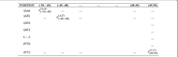
Construction of scoring matrices
For a sequence of lbp long, l-1 combinations of two adjacent positions are possible. Again, in each combination, 16 pairs of nucleotides (AA, AT,…,CG, CC) are possible. Thus, scoring matrices, each of order 16× (l-1), were constructed using di-nucleotide association scores under all the three procedures. Figure 5 shows a sample scoring matrix for 102 bp window length.
Ten-fold cross-validation and encoding of splice site sequence
TSS and FSS sequence datasets were separately divided into 10 random non-overlapping sets for the purpose of 10-fold cross validation. In each fold, one set of TSS and one set of FSS together were used as the test dataset and remaining 9 sets of
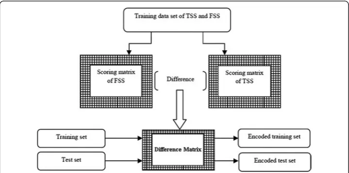
TSS and 9 sets of FSS together were used as the training dataset. This was performed because 10-fold cross validation procedure is a standard experimental technique for de-termining how well a classifier performs on a test data set [21]. For each training set, scoring matrices for TSS and FSS were constructed independently and then the differ-ence matrix was derived by subtracting the TSS scoring matrix from the FSS scoring matrix. The training and test datasets were then encoded by passing the corresponding sequences through the difference matrix (Fig. 6), where each sequence was transformed into a vector of scores of length l-1. A detailed explanation on encoding of the se-quence is provided in Additional file 1.
Classification using Random Forest
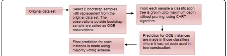
LetL(y, x) be the learning dataset, where x is a matrix ofnrows (observations) andp columns (variables), yis the response variable that takes values from Kclasses. Then, the RF consists of ensemble of B tree classifiers, where each classifier is constructed upon a bootstrap sample of the learning dataset. Each classifier of RF votes each test in-stances to one of the pre-defined Kclasses. Finally, each test instance is predicted by the label of winning class. As the individual trees are constructed upon a bootstrap sample, on an average 36.8 % 1−1
n
n
≈1
e;ðe≈2:718Þ
of instances do not play any role in the construction of each tree, and are called as Out Of Bag (OOB) instances. These OOB instances are the source of data used in RF for estimating the prediction error (Fig. 7). RF is computationally very efficient and offers high prediction accuracy with less sensitiveness to noisy data. For classification of TSS and FSS, RF was chosen over the other classifiers as it is a non-parametric (i.e., it does not make any assumption about the probability distribution of the dataset) method as well as its ability to handle large data sets. For more details about RF, one can refer [10].
Tuning of parameters
There are two important parameters in RF viz., number of variables to choose at each node for splitting (mtry) and number of trees to grow in the forest (ntree). Tuning of these parameters is required to achieve maximum prediction accuracy.
mtry
A small value of mtry produces less correlated trees that consequently results in lower variance of prediction. Though, integer (log2(p+1)) number of predictors per node has been recommended by Breiman [10], this mayn’t provide best possible result al-ways. Thus, RF model was executed with different mtry values i.e., 1, √p, 20%*p, 30%*p, 50%*pand p to find out the optimum one. The parameterization that gener-ated the lowest and stable OOB Error Rate (OOB-ER) was chosen as the optimalmtry.
ntree
Many times, the number of trees to be grown in the forest for getting the stable OOB-ER is not known. Moreover, OOB-ER is totally dependent on the type of data, where the stronger predictor leads to quicker convergence. Therefore, the RF was grown with different number of trees, and the number of trees after which the error rate got stabilized was considered as the optimalntree.
Margin function
Margin function is one of the important features of RF that measures the extent to which the average vote for right class exceeds the average vote for any other class. Let (x, y) be the training set havingn number of observations where each vector of attri-butes (x) is labeled with class yj(where, j = 1, 2 for binary class), i.e., the correct class is
denoted by y (either y1or y2). Further, let prob(yj) be the probability of class yj, then
the margin function of the labeled observation (x, y) is given by
mðx; yÞ ¼prob h½ ð Þ ¼x y− max j¼1 yj≠y
2
prob hð Þ ¼x yj
h i
If m(x, y) > 0, then h (x) correctly classifies y, where h(x) denotes a classifier that predicts the label y for an observation x. The value of margin function always lies between-1 to 1.
Implementation
The RF code was originally written in Fortran by Breiman and Cutler and also included as a package “randomForest” in R [22] and this package was implemented (for execu-tion of RF model) on a windows server (82/GHz and 32 GB memory). Run time was
dependent on data size and mtry, ranging from 1 second per tree to over 10 seconds per tree.
Performance metrics
The performance metrics viz., Sensitivity or True Positive Rate (TPR), Specificity or True Negative Rate (TNR), F-measure, Weighted Accuracy (WA), G-mean and Mat-thew’s Correlation Coefficient (MCC), all of which are the functions of confusion matrix, were used to evaluate the performance of RF. The confusion matrix contains information about the actual and predicted classes. Figure 8 shows the confusion matrix for a binary classifier, where TP is the number of TSS being predicted as TSS and TN is the number of FSS being predicted as FSS, FN is the number of TSS being incorrectly predicted as FSS and FP is the number of FSS being incorrectly predicted as TSS. The different performance metrics are defined as follows:
TPR or Sensitivity ¼ T P
T PþFN ðSame as recall f or binary classificationÞ
TNR or Specificity ¼ T N T NþFP
F−measureð Þα ¼ð1þαÞ recallprecision
αrecall
ð Þ þprecision ðαtakes discrete valuesÞ; Precision
¼ T P
T PþFP
F−measureð Þβ ¼ 1þβ
2
recallprecision
β2recall
þprecision ðβtakes discrete valuesÞ
WA¼1 2
T P T PþFNþ
T N T NþFP
G−Mean ¼
ffiffiffiffiffiffiffiffiffiffiffiffiffiffiffiffiffiffiffiffiffiffiffiffiffiffiffiffiffiffiffiffiffiffiffiffiffiffiffiffiffiffiffiffiffiffiffiffiffiffiffiffiffi T P
T PþFN
T N T NþFP
s
MCC¼ ffiffiffiffiffiffiffiffiffiffiffiffiffiffiffiffiffiffiffiffiffiffiffiffiffiffiffiffiffiffiffiffiffiffiffiffiffiffiffiffiffiffiffiffiffiffiffiffiffiffiffiffiffiffiffiffiffiffiffiffiffiffiffiffiffiffiffiffiffiffiffiffiffiffiffiffiffiffiffiffiffiffiffiffiffiffiffiffiffiffiffiffiðT PT NÞ−ðFPFNÞ T PþFP
ð ÞðT PþFNÞðT NþFPÞðT NþFNÞ p
Comparison of RF with SVM and ANN
The performances of RF was compared with that of SVM [23], ANN [24] using the same dataset that was used to analyze the performance of RF. The “e1071” [25] and “RSNNS”[26] packages of R software were used for implementing the SVM and ANN respectively. The SVM and ANN classifiers were chosen for comparison because these two techniques have been most commonly used for prediction purpose in the field of bioinformatics. In classification, SVM separates the different classes of data by a hyper-plane. In terms of classification performance, the optimal hyper-plane is the one that separates the classes with maximum margin (a clear gap as wide as possible). The sam-ple observations on the margins are called the support vectors that carry all the rele-vant information for classification [23]. ANNs are non-linear mapping structures based on the function of neural networks in the human brain. They are powerful tools for modeling especially when the underlying relationship is unknown. ANNs can identify and learn correlated patterns between input datasets and corresponding target values. After training, ANNs can be used to predict the outcome of new independent input data [24]. The SVM model was trained with the radial basis function (gamma = 0.01) as kernel. In the ANN model, multilayer perceptron was used with“Randomize_Weights” as initialization function, “Std_Backpropagation” as learning function and “ Act_Logis-tic”as hidden activation function. The 10-fold cross validation was performed for SVM and ANN, similar to RF. All the three techniques were then compared in terms of performance metrics. Also, the MCC values of RF, SVM and ANN were plotted to analyze the consistency over 10 folds of the cross validation. A similar kind of compari-son between RF, SVM and ANN was also made using the imbalanced dataset. To han-dle the imbalanced data, one additional parameter i.e., cutoff was used in RF, where 90 % cutoff was assigned to the major class (class having larger number of observations) i.e., FSS and 10 % to the minor class (class having lesser number of observations) i.e., TSS, based on the degree of imbalanced-ness in the dataset. Similarly, one additional parameter i.e.,class.weightswas used in SVM model, and the weights used were 19 and 1 for TSS and FSS respectively (keeping in view the proportion of TSS and FSS in the dataset). However, no parameter to handle imbalanced-ness was found in“RSNNS”package, there-fore the same model of ANN was trained using imbalanced data.
In the case of imbalanced test dataset, the performance metrics were computed by
assigning weights w1to TP & FN and w2to FP & TN. Here, w1 ¼n FSS.
nT SSþnFSS
ð Þ and
w2¼n TSS.
nT SSþnFSS
ð Þ, wheren
TSS
is the number of TSS andnFSSis the number of FSS in
the test dataset. Further, the Mann Whitney Utest at 5 % level of significance was per-formed to evaluate the difference among the prediction accuracies of RF, SVM and ANN, by using the statspackage of R-software.
Comparison with other prediction tools
Model of 1storder (MM1) and Weighted Matrix Method (WMM) given under MaxEntS-can were also used for comparison. The independent test set was prepared using two different genes (AF102137.1 and M63962.1) downloaded from Genbank (http:// www.ncbi.nlm.nih.gov/genbank/) randomly. Comparison among the approaches was made using the values of performance metrics.
Web server
A web server for the prediction of donor splice sites was developed using HTML and PHP. The developed R-code was executed in the background using PHP script upon the submission of sequences in FASTA format. The web page was designed to facilitate the user for a sequence input, selection of species (human) and encoding procedures. In the server, the model has been trained with human splice site data and the user has to supply only the test sequence (s) of his/her interest to predict the donor splice sites.
Results
Analysis of sequence distribution
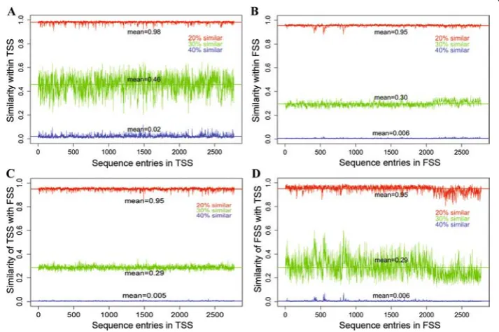
The removal of the identical sequences from the TSS dataset resulted in 2775 unique TSS. A graphical representation of degree of similarity within TSS, within FSS and be-tween TSS & FSS is shown in Fig. 9. It is observed that each sequence of TSS is 40 % (blue) similar with an average of 56 (0.02*2775) sequences of TSS (Fig. 9a) and 15 (0.005*2775) sequences of FSS (Fig. 9c). On the other hand, each sequence of FSS is 40 % (blue) similar with an average of 17 (0.006*2775) sequences of FSS (Fig. 9b) and 17 sequences of TSS (Fig. 9d). Similarly, each sequence of TSS is 30 % (green) similar
with an average of 1276 (0.46*2775) sequences of TSS (Fig. 9a) and 805 (0.29*2775) se-quences of FSS (Fig. 9c). On the other hand, each sequence of FSS is 30 % (green) simi-lar with an average of 832 (0.30*2775) sequences of FSS (Fig. 9b) and 805 (0.29*2775) sequences of TSS (Fig. 9d). Further, more than 90 % of sequences of entire dataset (both TSS and FSS) are observed to be at least 20 % similar with each other.
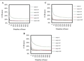
Optimum values of parameters
The graph of OOB error against ntree (500) for different mtry values is shown in Fig. 10. From Fig. 10 it is observed that the OOB errors are stabilized after 200 trees, for allmtryvalues and that too in all the three encoding procedures. Besides, it is observed that OOB error is minimum at mtry=50, irrespective of the encoding procedures. Hence, the optimum values of mtry and ntree were determined as 50 and 200 respectively. The final prediction was made with optimum values of the parameters.
Performance analysis of random forest
The plot of margin function for all the 10 folds of the cross-validation under P-1 is shown in Fig. 11. The points in red color in Fig. 11 indicate the predicted FSS and blue color indicate the predicted TSS. The same for P-2 and P-3 are provided in Add-itional files 2 and 3 respectively. The instances having the values of margin function greater than or equal to zero are correctly predicted test instances and less than zero are incorrectly predicted test instances. From Fig. 11 it is observed that most of the values of margin function are above zero both in TSS and FSS i.e., the RF achieved
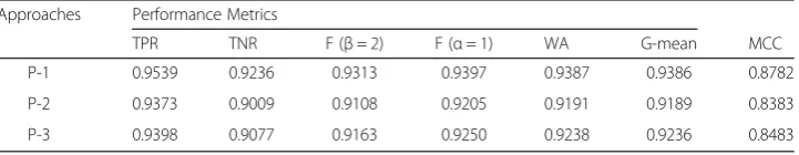
high prediction accuracy. Similar results are also found in case of P-2 and P-3. Fur-ther, the performance of RF is measured in terms of performance metrics and is pre-sented in Table 1. From Table 1 it is seen that the number of correctly predicted TSS is higher than that of FSS, in all the three encoding approaches. Also, it is observed that the average prediction accuracies are ~93 %, ~91 % and ~92 % under P-1, P-2 and P-3 respectively.
Fig. 11Graphical representation of margin functions for ten-fold cross-validation. Red color points for FSS and blue color for TSS. The instances having value of margin function greater than or equal to zero are correctly predicted test instances and instances having value below zero indicate incorrectly predicted test instances
Table 1Performance metrics of RF for three encoding procedures
Approaches Performance Metrics
TPR TNR F (β= 2) F (α= 1) WA G-mean MCC
P-1 0.9539 0.9236 0.9313 0.9397 0.9387 0.9386 0.8782
P-2 0.9373 0.9009 0.9108 0.9205 0.9191 0.9189 0.8383
Comparative analysis among different classifiers
The performance metrics of RF, SVM and ANN under P-1, P-2 and P-3 for both bal-anced and imbalbal-anced training datasets are presented in Table 2. The plots of MCC for RF, SVM and ANN are shown in Fig. 12. From Table 2 it is observed that the predic-tion accuracies of RF are higher than that of SVM and ANN under both balanced and imbalanced situations. It is further observed that for the balanced training dataset the performances of RF and SVM are not significantly different in P-1 but significantly dif-ferent in P-2 and P-3 (Table 3). However, the RF performed significantly better than that of ANN in all the three procedures. Furthermore, all the three classifiers achieved higher accuracies in case of balanced training dataset as compared to the imbalanced training dataset. Besides, RF achieved consistent accuracy over the 10 folds under all the three encoding procedures (Fig. 12). On the other hand, SVM and ANN could not achieve consistent accuracies in P-2 and P-3 over different folds of the cross validation.
Though RF performed better than SVM and ANN, its performance was further com-pared with that of Bagging [27], Boosting [28], Logistic regression [29], kNN [30] and Naïve Bayes [29] classifiers to assess its superiority. The functions bagging (), ada (), glm (),knn ()and NaiveBayes ()available in R-packages “class” [31],“klaR” [32],“stats” [33], “ada” [34] and “ipred” [35] were used to implement Bagging, Boosting, Logistic regression, kNN and Naïve Bayes classifiers respectively. The values of performance metrics, their standard errors and P-values for testing the significance are provided in Table 4, Table 5 and Table 6 respectively. It is observed that the performance of RF is not significantly different from that of Bagging and Boosting in case of balanced dataset (Table 6). On the contrary, RF outperformed both Bagging and Boosting classifiers under imbalanced situation (Table 6). It is also noticed that the classification accuracies (performance metrics) of RF are significantly higher than that of Logistic regression, kNN and Naïve Bayes classifiers under both the balanced and imbalanced situations (Table 4, Table 6).
Comparison of RF with other prediction tools
The performance metrics of the proposed approach and the considered existing methods computed by using an independent test dataset is presented in Table 7. It is seen that none of the existing approaches achieved above 90 % TPR. On the other hand, all other approaches (except SpliceView) achieved higher values of TNR than that of proposed approach (Table 7). Furthermore, the proposed approach achieved more than 90 % accuracy in terms of different performance metrics (Table 7).
Online prediction server-MaLDoSS
Table 2Comparison of the performance of RF, SVM and ANN under all encoding procedures with both balanced and imbalanced training dataset
EP MLA Balanced Dataset Imbalanced Dataset
TPR TNR F (α= 1) F (β= 2) G-mean WA MCC TPR TNR F (α= 1) F (β= 2) G-mean WA MCC
P-1 RF 0.954 0.924 0.940 0.932 0.939 0.939 0.878 0.842 0.896 0.865 0.880 0.869 0.869 0.739
(0.014) (0.014) (0.010) (0.012) (0.010) (0.010) (0.020) (0.064) (0.018) (0.032) (0.049) (0.030) (0.028) (0.043)
SVM 0.935 0.930 0.933 0.931 0.933 0.933 0.865 0.104 0.982 0.185 0.349 0.320 0.543 0.180
(0.015) (0.017) (0.015) (0.015) (0.016) (0.016) (0.031) (0.027) (0.018) (0.041) (0.031) (0.040) (0.013) (0.061)
ANN 0.892 0.896 0.894 0.895 0.894 0.894 0.787 0.032 0.988 0.061 0.136 0.178 0.510 0.068
(0.064) (0.080) (0.063) (0.062) (0.066) (0.065) (0.129) (0.026) (0.010) (0.046) (0.032) (0.065) (0.011) (0.055)
P-2 RF 0.937 0.901 0.920 0.911 0.919 0.919 0.838 0.883 0.894 0.888 0.891 0.888 0.889 0.777
(0.020) (0.016) (0.016) (0.018) (0.016) (0.016) (0.033) (0.038) () (0.025) (0.030) (0.019) (0.019) (0.035)
SVM 0.720 0.773 0.740 0.752 0.746 0.746 0.493 0.321 0.989 0.482 0.689 0.563 0.655 0.417
(0.029) (0.106) (0.041) (0.026) (0.049) (0.051) (0.108) (0.051) (0.008) (0.055) (0.053) (0.043) (0.025) (0.048)
ANN 0.775 0.777 0.776 0.776 0.776 0.776 0.552 0.305 0.978 0.460 0.661 0.546 0.642 0.383
(0.067) (0.037) (0.049) (0.059) (0.048) (0.045) (0.090) (0.049) (0.014) (0.052) (0.051) (0.043) (0.022) (0.046)
P-3 RF 0.940 0.908 0.925 0.917 0.924 0.924 0.848 0.879 0.891 0.884 0.888 0.885 0.885 0.770
(0.017) (0.015) (0.012) (0.014) (0.012) (0.012) (0.246) (0.044) (0.022) (0.029) (0.034) (0.022) (0.022) (0.042)
SVM 0.789 0.807 0.796 0.800 0.798 0.798 0.595 0.249 0.988 0.395 0.609 0.496 0.619 0.352
(0.044) (0.068) (0.042) (0.042) (0.046) (0.045) (0.090) (0.052) (0.008) (0.062) (0.056) (0.049) (0.026) (0.055)
ANN 0.757 0.760 0.758 0.759 0.759 0.759 0.517 0.272 0.979 0.421 0.626 0.516 0.626 0.355
(0.118) (0.099) (0.067) (0.098) (0.057) (0.048) (0.086) (0.066) (0.009) (0.081) (0.072) (0.064) (0.034) (0.076) The values inside the brackets () are the standard errors
EPencoding procedure,MLAmachine learning approaches
BioData
Mining
(2016) 9:4
Page
15
of
Discussion
Many statistical methods like, Back Propagation Neural Networks (BPNN), Markov Model, SVM etc. have been used for prediction of ss in the past. Rajapakse and CaH [4] introduced a complex ss prediction system (combination of 2nd order Markov model and BPNN) that achieved higher prediction accuracy than that of Genesplicer [36], but at the same time it is required longer sequence motifs to train the model. Moreover, BPNN is computationally expensive and may increase further with the inclu-sion of 2ndorder Markov model. Baten et al. [6] reported improved prediction accuracy by using SVM with Salzberg kernel [37], where the empirical estimates of conditional positional probabilities of the nucleotides around the splicing junctions are used as in-put in SVM. Sonnenburg et al. [7] employed weighted degree kernel method in SVM for the genome-wide recognition ofss, which is based on complex nonlinear transform-ation. In the present study we applied RF as it is computationally feasible and user friendly. Furthermore, the fine tuning of parameters of RF helps in improving the pre-diction accuracy.
Most of the existing methods capture position specific signals as well as nucleotide dependencies for the prediction ofss. In particular, Roca et al. [9] explained the pivotal role played by the nucleotide dependencies for the prediction of donor ss. Therefore,
the proposed encoding procedures are based on di-nucleotide dependencies. Further, the earlier ss prediction methods such as Weighted Matrix Method (WMM) [38], Weighted Array Model (WAM) [39] and Maximal Dependency Decomposition (MDD) [40] only considered the TSS but not the FSS to train the prediction model. However, FSS are also necessary [41], and hence RF was trained with both TSS and FSS datasets.
There is a chance of occurrence of same ss motifs in both TSS and FSS when the length ofssmotif is small. To avoid such ambiguity, instead of 9 bp long motif (3 from exons and 6 from introns) [42], the longerssmotif (102 bp long) was considered in this study. Further, duplicate sequences were removed and a similarity search was per-formed to analyze the sequence distribution. It is found that each sequence of TSS is 40 % similar with an average of 0.5 % sequences of FSS (Fig. 9c) and each sequence of FSS is 40 % similar with an average of 0.6 % sequences of TSS (Fig. 9d). Also, the se-quences are found to be similar (20 % similarity) within the classes (Fig. 9a-b). This im-plies that the presence of within class dissimilarities and between class similarities in the dataset. Thus the performance of the proposed approach is not over estimated.
The procedure followed in the present study includes WMM and WAM procedures to some extent in finding the weights for the first order dependencies. Besides, the difference matrix captured the difference in the variability pattern existing among the adjacent di-nucleotides in the TSS and FSS. Li et al. [43] have also used di-nucleotide frequency difference as one of the positional feature in prediction ofss.
The optimum value of mtry was observed as 50, determined on the basis of lowest and stable OOB-ER. This may be due to the fact that each position was represented twice (except the 1stand 102nd positions) in the set of 101 variables (1_2, 2_3, 3_4,…,
Table 3P-values of Mann Whitney U statistic for testing the significant difference between
RF-SVM, RF-ANN and SVM-ANN at 5 % level of significance for all the performance measures under both balanced and imbalanced training datasets
$D EP MLA TPR TNR F (α= 1) F (β= 2) G-mean WA MCC
Table 4Performance metrics of Bagging, Boosting, Logistic regression,kNN and Naïve Bayes classifiers for all the three encoding procedures under both balanced and imbalanced situations
EP MD Balanced Imbalanced
TPR TNR F (α= 1) F (β= 2) G-mean WA MCC TPR TNR F (α= 1) F (β= 2) G-mean WA MCC
P-1 BG 0.944 0.921 0.934 0.940 0.933 0.933 0.866 0.069 0.996 0.127 0.084 0.258 0.533 0.172
BS 0.952 0.919 0.936 0.945 0.935 0.935 0.872 0.041 0.898 0.079 0.051 0.192 0.470 0.129
LG 0.895 0.882 0.889 0.892 0.888 0.888 0.777 0.008 0.993 0.016 0.010 0.087 0.502 0.012
NB 0.835 0.836 0.836 0.835 0.834 0.835 0.674 0.202 0.838 0.297 0.231 0.409 0.520 0.067
KN 0.856 0.840 0.847 0.852 0.847 0.848 0.697 0.048 0.854 0.087 0.058 0.200 0.451 0.012
P-2 BG 0.927 0.882 0.907 0.919 0.904 0.904 0.810 0.112 0.992 0.198 0.135 0.330 0.552 0.216
BS 0.934 0.901 0.918 0.928 0.917 0.917 0.835 0.090 0.996 0.163 0.109 0.296 0.543 0.200
LG 0.742 0.734 0.739 0.741 0.737 0.738 0.478 0.112 0.981 0.198 0.135 0.330 0.547 0.190
NB 0.772 0.758 0.767 0.770 0.764 0.765 0.532 0.159 0.884 0.250 0.186 0.373 0.521 0.073
KN 0.813 0.678 0.760 0.790 0.739 0.746 0.502 0.173 0.981 0.290 0.207 0.412 0.577 0.262
P-3 BG 0.924 0.904 0.915 0.920 0.914 0.914 0.828 0.125 0.991 0.220 0.151 0.351 0.558 0.230
BS 0.941 0.898 0.922 0.933 0.920 0.920 0.841 0.095 0.995 0.171 0.115 0.305 0.545 0.205
LG 0.813 0.775 0.798 0.807 0.793 0.794 0.589 0.120 0.983 0.210 0.144 0.342 0.551 0.202
NB 0.784 0.761 0.775 0.780 0.771 0.772 0.547 0.178 0.945 0.289 0.210 0.410 0.562 0.196
KN 0.795 0.700 0.756 0.778 0.742 0.747 0.501 0.065 0.989 0.120 0.080 0.247 0.527 0.142
MDmethods,EPencoding procedures,BGbagging,BSboosting,LGlogistic regression,NBnaïve bayes,KN Knearest neighbor
BioData
Mining
(2016) 9:4
Page
18
of
Table 5Standard errors of different performance metrics for Bagging, Boosting, Logistic regression,kNN and Naïve Bayes classifiers for all the three encoding procedures under both balanced and imbalanced situations
EP MD Balanced Imbalanced
TPR TNR F (α= 1) F (β= 2) G-mean WA MCC TPR TNR F (α= 1) F (β= 2) G-mean WA MCC
P-1 BG 0.0201 0.0178 0.0114 0.0156 0.0113 0.0113 0.0226 0.0234 0.0036 0.0409 0.0282 0.0474 0.0108 0.0334 BS 0.0146 0.0149 0.0111 0.0125 0.0113 0.0112 0.0224 0.0177 0.3156 0.0334 0.0218 0.0715 0.1652 0.0504 LG 0.0569 0.0740 0.0601 0.0575 0.0624 0.0621 0.1238 0.0065 0.0056 0.0121 0.0076 0.0313 0.0045 0.0267 NB 0.0630 0.0826 0.0560 0.0571 0.0573 0.0577 0.1169 0.0357 0.1043 0.0500 0.0390 0.0439 0.0549 0.1579 KN 0.1502 0.1279 0.1386 0.1454 0.1364 0.1354 0.2701 0.0221 0.3023 0.0389 0.0267 0.0765 0.1595 0.0799 P-2 BG 0.0201 0.0272 0.0192 0.0188 0.0201 0.0200 0.0397 0.0261 0.0060 0.0429 0.0310 0.0421 0.0130 0.0364 BS 0.0207 0.0179 0.0161 0.0184 0.0163 0.0163 0.0327 0.0273 0.0033 0.0456 0.0325 0.0461 0.0134 0.0358 LG 0.0688 0.0799 0.0617 0.0644 0.0630 0.0632 0.1272 0.0182 0.0148 0.0290 0.0214 0.0273 0.0107 0.0410 NB 0.0546 0.0629 0.0421 0.0472 0.0405 0.0407 0.0824 0.0316 0.0733 0.0487 0.0363 0.0436 0.0426 0.1342 KN 0.0925 0.0811 0.0362 0.0681 0.0266 0.0280 0.0598 0.0235 0.0044 0.0337 0.0269 0.0282 0.0117 0.0270 P-3 BG 0.0156 0.0186 0.0117 0.0130 0.0120 0.0119 0.0237 0.0185 0.0052 0.0291 0.0217 0.0267 0.0089 0.0235 BS 0.0121 0.0178 0.0102 0.0102 0.0108 0.0107 0.0210 0.0194 0.0039 0.0324 0.0231 0.0323 0.0095 0.0256 LG 0.0406 0.0586 0.0376 0.0377 0.0409 0.0402 0.0795 0.0210 0.0116 0.0334 0.0247 0.0303 0.0132 0.0440 NB 0.0380 0.0689 0.0330 0.0323 0.0372 0.0368 0.0735 0.0254 0.0434 0.0397 0.0295 0.0333 0.0286 0.0913 KN 0.1017 0.0829 0.0629 0.0842 0.0566 0.0544 0.1076 0.0292 0.0078 0.0504 0.0352 0.0629 0.0116 0.0334 MDmethods,EPencoding procedures,BGbagging,BSboosting,LGlogistic regression,NBnaïve bayes,KN Knearest neighbor
BioData
Mining
(2016) 9:4
Page
19
of
Table 6P-values of the Mann Whitney statistic to test the significant difference between the performance of RF with that of Bagging, Boosting, Logistic regression,kNN and Naïve Bayes classifiers in all the three encoding procedures under both balanced and imbalanced situations
$D EP CLs TPR TNR F (α= 1) F (β= 2) G-mean WA MCC
Balanced P-1 RF-BG 0.343066 0.676435 0.272856 0.212122 0.185711 0.240436 0.272856 RF-BS 0.820063 0.939006 0.314999 0.795936 0.314999 0.383598 0.314999 RF-LG 0.001672 0.053092 0.002879 0.000725 0.005196 0.009082 0.005196 RF-NB 0.000242 0.002796 1.08E-05 1.08E-05 1.08E-05 0.000181 1.08E-05 RF-KN 0.053182 0.087051 0.028806 0.063013 0.035463 0.025581 0.028806 P-2 RF-BG 0.41319 0.594314 0.356232 0.356232 0.277512 0.315378 0.356232 RF-BS 0.837765 0.367844 0.968239 0.968239 0.842105 0.743537 0.842105 RF-LG 0.000275 0.000439 2.17E-05 2.17E-05 2.17E-05 2.17E-05 2.17E-05 RF-NB 0.000275 0.004216 2.17E-05 2.17E-05 2.17E-05 2.17E-05 2.17E-05 RF-KN 0.000376 0.000273 2.17E-05 2.17E-05 2.17E-05 0.000278 2.17E-05 P-3 RF-BG 0.171672 0.879378 0.14314 0.14314 0.165494 0.15062 0.14314
RF-BS 0.494174 0.381613 0.970512 0.528849 0.853428 0.820197 0.911797 RF-LG 0.000181 0.000181 1.08E-05 1.08E-05 1.08E-05 1.08E-05 1.08E-05 RF-NB 0.000182 0.000279 1.08E-05 1.08E-05 1.08E-05 0.000182 1.08E-05 RF-KN 0.000182 0.000181 1.08E-05 1.08E-05 1.08E-05 0.000182 1.08E-05 Imbalanced P-1 RF-BG 0.000269 0.000251 2.17E-05 2.17E-05 2.17E-05 0.000278 2.17E-05 RF-BS 0.000176 0.002555 0.000181 0.000181 0.000181 0.000178 0.000181 RF-LG 0.000263 0.000268 2.17E-05 2.17E-05 2.17E-05 0.000263 2.17E-05 RF-NB 0.000271 0.177338 2.17E-05 2.17E-05 2.17E-05 2.17E-05 2.17E-05 RF-KN 0.000175 0.025526 1.08E-05 1.08E-05 1.08E-05 0.000182 0.000179 P-2 RF-BG 0.000179 0.000173 0.000182 0.000182 0.000182 0.000181 0.000182 RF-BS 0.000181 0.000158 1.08E-05 1.08E-05 1.08E-05 0.000181 1.08E-05 RF-LG 0.00018 0.000178 1.08E-05 1.08E-05 1.08E-05 0.00018 1.08E-05 RF-NB 0.000182 0.733634 1.08E-05 1.08E-05 1.08E-05 0.000182 1.08E-05 RF-KN 0.000181 0.000174 1.08E-05 1.08E-05 1.08E-05 0.000182 1.08E-05 P-3 RF-BG 0.000176 0.000168 0.000182 0.000182 0.000182 0.000181 0.000182 RF-BS 0.000179 0.000149 1.08E-05 1.08E-05 1.08E-05 1.08E-05 1.08E-05 RF-LG 0.000179 0.000177 1.08E-05 1.08E-05 1.08E-05 0.000182 1.08E-05 RF-NB 0.000177 0.009082 1.08E-05 1.08E-05 1.08E-05 1.08E-05 1.08E-05 RF-KN 0.00018 0.00018 1.08E-05 1.08E-05 1.08E-05 0.000178 1.08E-05 $Ddata type,RFrandom forest, CLs classifiers,BGbagging,BSboosting,LGlogistic regression,NBnaïve bayes,KN K nearest neighbor
Table 7The performance metrics for the proposed approach and other published tools using the
independent test set
Methods TPR TNR F (α= 1) F (β= 2) G-mean WA MCC
MaxEntScan 0.627 0.990 0.766 0.884 0.788 0.809 0.662
MDD 0.651 0.991 0.784 0.894 0.803 0.821 0.682
MM1 0.581 0.988 0.730 0.862 0.758 0.785 0.623
WMM 0.415 0.986 0.581 0.764 0.640 0.701 0.488
NNSplice 0.733 0.954 0.824 0.891 0.837 0.844 0.705
SpliceView 0.888 0.879 0.884 0.882 0.883 0.884 0.767
100_101, 101_102). Further, OOB-ER was found to be stabilized with small number of trees (ntree= 200) and this may be due to the existence of di-nucleotide dependencies in the ss motifs that leads to the high correlation between trees grown in the forest. However, we considered thentree equal to 1000 as (i) the computational time was not much higher than that required forntree=200, and (ii) the prediction accuracy may in-crease with inin-crease in the number of trees. Hence, the final RF model was executed withmtry= 50 andntree= 1000. The classification accuracy of RF model was measured in terms of margin function, over 10 folds of cross-validation. It is found that the prob-ability of instances being predicted as the correct class over the wrong class is very high (Fig. 11), which is a strong indication that the proposed approach with RF classifier is well defined and capable of capturing the variability pattern in the dataset.
As far as the encoding procedures are concerned, it is analyzed that the dependencies between the adjacent nucleotide positions in the sspositively influenced the prediction accuracy. Out of the three procedures (P-1, P-2 and P-3), P-1 is found to be superior with respect to different performance metrics. Though the accuracy of P-2 is observed to be lower than that of P-3, the difference is negligible. Therefore, it is inferred that the ratio of the observed frequency to the random frequency of di-nucleotide is an im-portant feature for discriminating TSS from FSS.
Among the classifiers, RF achieved above 91 % accuracy in all the three encoding procedures, while SVM showed a similar trend only for P-1 and ANN could not achieve above 90 % under any of the encoding procedures (Table 2). The MCC values of RF, SVM and ANN also supported the above finding. Though SVM and ANN per-formed well in P-1, their consistencies were relatively low in P-2 and P-3 over 10 folds
of cross validation. On the other hand, RF was found to be more consistent in all the three encoding procedures. Further, the prediction accuracy of RF was not significantly different (P-value > 0.05) from that of SVM, whereas it was significantly higher (P-value < 0.05) than that of ANN in balanced training set under P-1. However, under P-2 and P-3, RF performed significantly better than that of SVM and ANN in both balanced and imbalanced situations (Table 3). Further, the performance of SVM was not signifi-cantly different than that of ANN in P-1, whereas it was signifisignifi-cantly different in P-2 and P-3 under both balanced and imbalanced datasets (Table 3). In case of imbalanced dataset, RF performed better than SVM and ANN in terms of sensitivity and overall ac-curacy (Table 2). Besides, the performances of SVM and ANN were biased towards the major class (FSS) whereas RF performed in an unbiased way. Furthermore, all the clas-sifiers performed better under P-2 and P-3 as compared to P-1, in case of imbalanced dataset (Table 2).
Besides SVM and ANN, the performance of Bagging, Boosting, Logistic regression, kNN and Naïve Bayes classifiers were also compared with that of RF. Though the per-formance of RF was found at par with that of Bagging and Boosting in balanced situ-ation, it was significantly higher than that of Logistic regression,kNN and Naïve Bayes classifiers. However, in case of imbalanced dataset, RF performed significantly better than Bagging, Boosting, Logistic regression, kNN and Naïve Bayes classifiers in all the three encoding procedures. Thus, RF can be considered as a better classifier over the others.
RF achieved highest prediction accuracy under P-1 as compared to the other combi-nations of encoding procedures (P-2, P-3) and classifiers (SVM, ANN, Bagging, Boost-ing, Logistic regression, kNN and Naïve Bayes). Therefore, the performance of RF under P-1 was compared with different existing tools i.e., MaxEntScan (Maximim Entropy Model, MDD, MM, WMM), SpliceView and NNSplice using an independent
test set. The overall accuracy of the proposed approach (RF with P-1) was found better than that of other considered (existing) tools.
The purpose of developing the web server is to facilitate easy prediction of donor splice sites by the users working in the area of genome annotations. The developed web server provides flexibility to the users for selecting the encoding procedures and the machine learning classifiers. As the test sequences belong to two different classes, the instances with probability >0.5 are expected to be true splice sites. Besides, higher the probability more is the strength of instance being a donor splice site. Though, the RF achieved higher accuracy under P-1 as compared to the other combinations, all combinations are provided in the server for the purpose of comparative analysis by the user. To our limited knowledge, for the first time, we have used RF inssprediction.
Conclusion
This paper presents a novel approach for donor splice site prediction that involves three splice site encoding procedures and application of RF methodology. The proposed ap-proach discriminated the TSS from FSS with higher accuracy. Also, the RF outperformed SVM, ANN, Bagging, Boosting, Logistic regression, kNN and Naïve Bayes classifiers in terms of prediction accuracy. Further, RF with the proposed encoding procedures showed high prediction accuracy both in balanced and imbalanced situations. Being a supplement to the commonly usedssprediction methods, the proposed approach is believed to con-tribute to the prediction of eukaryotic gene structure. The web server will help the user for easy prediction of donorss.
Availability and requirement
MaLDoSS, the donor splice site prediction server, is freely accessible to the non-profit and academic biological community for research purposes at http://cabgrid.res.in:8080/ maldoss.
Additional files
Additional file 1:An example of the proposed sequence encoding approach.Description of the data: A precise description about the sequence encoding procedure is provided with an example. (PDF 72 kb)
Additional file 2:Plotting of margin function for encoding procedure 2 (P-2).Description of the data: Each dot in the plot is the value of margin function for an observation (TSS or FSS). Ten different plots corresponding to 10 test sets of the 10-fold cross validation. Red and blue points are the values of margin function for FSS and TSS. The values above zero indicate that the instances are correctly classified. (PDF 110 kb)
Additional file 3:Plotting of margin function for encoding procedure 3 (P-3).Description of the data: Each dot in the plot is the value of margin function for an observation (TSS or FSS). Ten different plots corresponding 10 test sets of the 10-fold cross validation. Red and blue points are the values of margin function for FSS and TSS. The values above zero indicate that the instances are correctly classified. (PDF 108 kb)
Abbreviations
ANN:artificial neural network; BPNN: back propagation neural network; EP: encoding procedure; FN: false negative; FSS: false splice sites; HS3D: homo sapiens splice dataset; MCC: matthew’s correlation coefficient; MDD: maximal dependency decomposition; MEM: maximum entropy modeling; MLA: machine learning approaches; MM1: markov model of 1storder; MM2: markov model of 2ndorder; OOB: out of bag; OOB-ER: out of bag-error rate;
PWM: position weight matrix; RF: random forest; SVM: support vector machine; TNR: true negative rate; TP: true positive; TPR: true positive rate; TSS: true splice sites; WA: weighted accuracy; WAM: weighted array model; WMM: weighted matrix model.
Competing interests
Authors’contributions
PKM and TKS collected the data, developed and implemented the methodology and drafted the manuscript. TKS and PKM developed the web server. ARR conceived the study and finalized the manuscript. All authors read and approved the final manuscript.
Acknowledgements
The grant (Agril. Edn.4-1/2013-A&P dated 11.11.2014) received from Indian Council of Agriculture Research (ICAR) for Centre for Agricultural Bioinformatics (CABin) scheme of Indian Agricultural Statistics Research Institute (IASRI) is duly acknowledged.
Author details
1Division of Statistical Genetics, Indian Agricultural Statistics Research Institute, New Delhi 110 012, India.2Centre for
Agricultural Bioinformatics, Indian Agricultural Statistics Research Institute, New Delhi 110 012, India.
Received: 2 March 2015 Accepted: 19 January 2016
References
1. Sheth N, Roca X, Hastings ML, Roeder T, Krainer AR, Sachidanandam R. Comprehensive splice site analysis using comparative genomics. Nucleic Acids Res. 2006;34:3955–67.
2. Chen TM, Lu CC, Li WH. Prediction of splice sites with dependency graphs and their expanded Bayesian networks. Bioinformatics. 2005;21(4):471–82.
3. Reese MG. Application of a time-delay neural network to promoter annotation in the Drosophila melanogaster genome. Comput Chem. 2001;26(1):51–6.
4. Rajapakse J, CaH LS. Markov encoding for detecting signals in genomic sequences. IEEE Trans Comput. Biol Bioinformatics. 2005;2(2):131–42.
5. Zhang XF, Katherine HA, Ilana HC, Lawrene LS, Chasin A. Sequence Information for the Splicing of Human Pre-mRNA Identified by Support Vector Machine Classification. Genome Res. 2003;13:2637–50.
6. Baten A, Chang B, Halgamuge S, Li J. Splice site identification using probabilistic parameters and SVM classification. BMC Bioinformatics. 2006;7 Suppl 5:S15.
7. Sören Sonnenburg S, Schweikert G, Philips P, Behr J, Rätsch G. Accurate splice site prediction using support vector machines. BMC Bioinformatics. 2007;8 Suppl 10:S7.
8. Yeo G, Burge CB. Maximum entropy modeling of short sequence motifs with applications to RNA splicing signals. J Comput Biol. 2004;11(2-3):377–94.
9. Roca X, Olson AJ, Rao AR, Enerly E, Kristensen VN, Børresen-Dale AL, et al. Features of 5′-splice-site efficiency derived from disease-causing mutations and comparative genomics. Genome Res. 2008;18:77–87. 10. Breiman L. Random Forests. Mach Learn. 2001;45:5–32.
11. Hamby SE, Hirst JD. Prediction of glycosylation sites using random forests. BMC Bioinformatics. 2008;9(1):500. 12. Jain P, Garibaldi JM, Hirst JD. Supervised machine learning algorithms for protein structure prediction. Comput
Biol Chem. 2009;33:216–23.
13. Dehzangi A, Phon-Amnuaisuk A, Dehzangi O. Using random forest for protein fold prediction problem: An empirical study. J Inf Sci Eng. 2010;26(6):1941–56.
14. Khalilia M, Chakraborty S, Popescu M. Predicting disease risk from highly imbalanced data using random forest. BMC Med Inform Decis Mak. 2011;11:51.
15. Pollastro P, Rampone S. HS3D: Homosapiens Splice Site Data Set. Nucleic Acids Res. 2003;100:15688–93. Annual Database Issue 36.
16. Blencowe BJ. Exonic splicing enhancers: mechanism of action, diversity and role in human genetic diseases. Trends Biochem Sci. 2000;25(3):106–10.
17. Lam BJ, Hertel KJ. A general role for splicing enhancers in exon definition. RNA. 2002;8(10):1233–41.
18. Zhao X, Huang H, Speed TP. Finding short DNA motifs using permuted Markov models. J Comput Biol. 2005; 12(6):894–906.
19. Dominski Z, Kole R. Selection of splice sites in pre-mRNAs with short internal exons. Mol Cell Biol. 1991; 11(12):6075–83.
20. Zhu J, He F, Wang D, Liu K, Huang D, Xiao J, et al. A Novel Role for Minimal Introns: Routing mRNAs to the Cytosol. PLoS One. 2010;5(4), e10144.
21. Stone M. Cross-validatory choice and assessment of statistical predictions. J Roy Statist Soc Ser B. 1974;36:111–47. 22. Liaw A, Wiener M. Prediction and regression by randomForest. Rnews. 2002;2:18–22.
23. Cortes C, Vapnik V. Support-Vector Networks. Mach Learn. 1995;20:273–97.
24. Haykin S. Neural Networks: a comprehensive foundation. Prentice Hall: Upper Saddle River; 1999. 25. Meyer D, Dimitriadou E, Hornik K, Weingessel A, Leisch F, et al. e1071: Misc functions of the Department of
Statistics (e1071), TU Wien, R package version 1.6-1. 2012.
26. Bergmeir C, Ben’ıtez JM. Neural Networks in R Using the Stuttgart Neural Network Simulator: RSNNS. J Stat Softw. 2012;46(7):1–26.
27. Breiman L: Bagging predictors. Technical Report 421, Department of Statistics, UC Berkeley, 1994. http://statistics. berkeley.edu/sites/default/files/tech-reports/421.pdf.
28. Drucker H, Cortes C, Jackel LD, LeCun Y, Vapnik V. Boosting and other ensemble methods. Neural Comput. 1994; 6(6):1289–301.
29. Mitchell T. Machine Learning. New York: McGraw Hill; 1997.
30. Hand D, Mannila H, Smyth P. Principles of Data Mining. Cambridge, MA: MIT Press; 2001.
32. Weihs C, Ligges U, Luebke K, Raabe N. klaR Analyzing German Business Cycles. In: Baier D, Decker R, Schmidt-Thieme L, editors. Data Analysis and Decision Support. Berlin: Springer; 2005. p. 335–43.
33. R Development Core Team: R: A language and environment for statistical computing. R Foundation for Statistical Computing, Vienna, Austria, 2012. ISBN 3-900051-07-0, URL http://www.R-project.org/
34. Culp M, Johnson K, Michailidis G: ada: an R package for stochastic boosting. R package version 2.0-3, 2012. http:// CRAN.R-project.org/package=ada.
35. Peters A, Hothorn T: ipred: Improved Predictors. R package version 0.9-3, 2013. http://CRAN.R-project.org/package=ipred. 36. Pertea M, Lin X, Salzberg SL. GeneSplicer: a new computational method for splice sites prediction. Nucleic Acids
Res. 2001;29(5):1185–90.
37. Zien A, Rätsch G, Mika S, Schölkopf B, Lengauer T, Müller KR. Engineering Support Vector Machine Kernels That Recognize Translation Initiation Sites. Bioinformatics. 2000;16(9):799–807.
38. Staden R. Computer methods to locate signals in nucleic acid sequences. Nucleic Acids Res. 1984;12:505–19. 39. Zhang MQ, Marr TG. A weight array method for splicing signal analysis. Comp Appl Biosci. 1993;9(5):499–509. 40. Burge C, Karlin S. Prediction of complete gene structures in human genomic DNA. J Mol Biol. 1997;268:78–94. 41. Huang J, Li T, Chen K, Wu J. An approach of encoding for prediction of splice sites using SVM. Biochimie.
2006;88:923–9.
42. Yin MM, Wang JTL. Effective hidden Markov models for detecting splicing junction sites in DNA sequences. Inform Sciences. 2001;139:139–63.
43. Li JL, Wang LF, Wang HY, Bai LY, Yuan ZM. High-accuracy splice sites prediction based on sequence component and position features. Genet Mol Res. 2012;11(3):3432–51.
• We accept pre-submission inquiries
• Our selector tool helps you to find the most relevant journal
• We provide round the clock customer support
• Convenient online submission
• Thorough peer review
• Inclusion in PubMed and all major indexing services
• Maximum visibility for your research
Submit your manuscript at www.biomedcentral.com/submit