Erik Forseth,1 Charles R. Evans,1 and Seth Hopper2, 3
1
Department of Physics and Astronomy, University of North Carolina, Chapel Hill, North Carolina 27599, USA 2School of Mathematics and Statistics and Complex & Adaptive Systems Laboratory,
University College Dublin, Belfield, Dublin 4, Ireland 3
CENTRA, Departamento de F´ısica, Instituto Superior T´ecnico IST, Avenida Rovisco Pais 1, 1049, Lisboa, Portugal
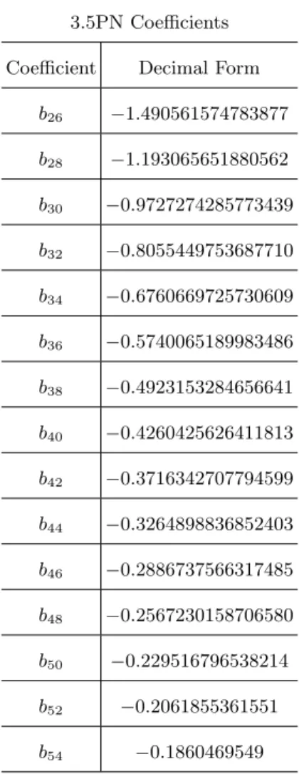
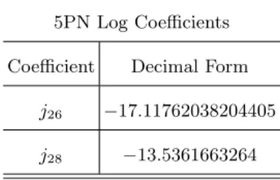
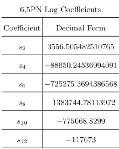
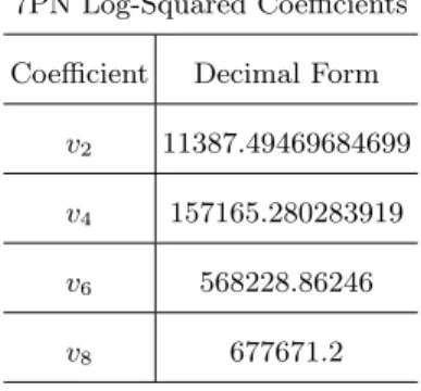
We present new results through 7PN order on the energy flux from eccentric extreme-mass-ratio binaries. The black hole perturbation calculations are made at very high accuracy (200 decimal places) using a Mathematica code based on the Mano-Suzuki-Takasugi (MST) analytic function expansion formalism. All published coefficients in the expansion through 3PN order at lowest order in the mass ratio are confirmed and new analytic and numeric terms are found to high order in powers of e2 at post-Newtonian orders between 3.5PN and 7PN. We also show original work in finding (nearly) arbitrarily accurate expansions for hereditary terms at 1.5PN, 2.5PN, and 3PN orders. An asymptotic analysis is developed that guides an understanding of eccentricity singular factors, which diverge at unit eccentricity and which appear at each PN order. We fit to a model at each PN order that includes these eccentricity singular factors, which allows the flux to be accurately determined out toe→1.
PACS numbers: 04.25.dg, 04.30.-w, 04.25.Nx, 04.30.Db
I. INTRODUCTION
Merging compact binaries have long been thought to be promising sources of gravitational waves that might be detectable in ground-based (Advanced LIGO, Advanced VIRGO, KAGRA, etc) [1–3] or space-based (eLISA) [4] experiments. With the first observation of a binary black hole merger (GW150914) by Advanced LIGO [5], the era of gravitational wave astronomy has arrived. This first observation emphasizes what was long understood– that detection of weak signals and physical parameter estimation will be aided by accurate theoretical pre-dictions. Both the native theoretical interest and the need to support detection efforts combine to motivate research in three complementary approaches [6] for com-puting merging binaries: numerical relativity [7, 8], post-Newtonian (PN) theory [9, 10], and gravitational self-force (GSF)/black hole perturbation (BHP) calculations [6, 11–14]. The effective-one-body (EOB) formalism then provides a synthesis, drawing calibration of its parame-ters from all three [15–20].
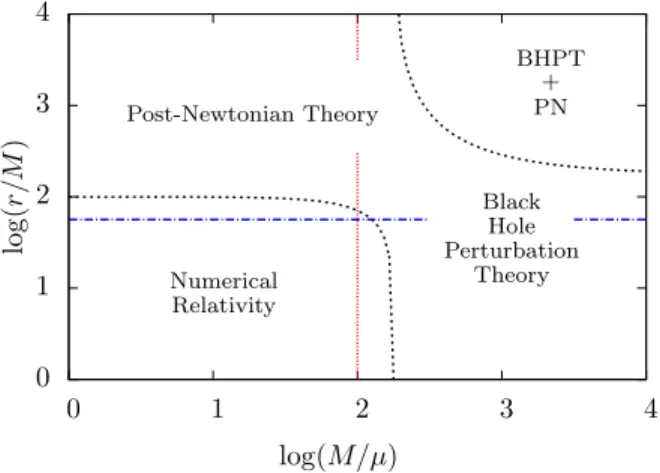
In the past seven years numerous comparisons [21– 30] have been made in the overlap region (Fig. 1) be-tween GSF/BHP theory and PN theory. PN theory is accurate for orbits with wide separations (or low fre-quencies) but arbitrary component masses, m1 and m2. The GSF/BHP approach assumes a small mass ratio q=m1/m2 1 (notation typically being m1=µ with black hole mass m2 = M). While requiring small q, GSF/BHP theory has no restriction on orbital separa-tion or field strength. Early BHP calculasepara-tions focused on comparing energy fluxes; see for example [31–34] for waves radiated to infinity from circular orbits and [35] for flux absorbed at the black hole horizon. Early cal-culations of losses from eccentric orbits were made by [36–39]. More recently, starting with Detweiler [21], it became possible with GSF theory to compare
conserva-0 1 2 3 4
0 1 2 3 4
log
(
r/
M
)
log(M/µ) Post-Newtonian Theory
Numerical Relativity
Black Hole Perturbation
Theory BHPT
+ PN
FIG. 1. Regions of binary parameter space in which different formalisms apply. Post-Newtonian (PN) approximation ap-plies best to binaries with wide orbital separation (or equiva-lently low frequency). Black hole perturbation (BHP) theory is relevant for binaries with small mass ratioµ/M. Numerical relativity (NR) works best for close binaries with comparable masses. This paper makes comparisons between PN and BHP results in their region of mutual overlap.
tivegauge-invariant quantities [22–25, 27, 29, 30, 40–42]. With the advent of extreme high-accuracy GSF calcula-tions [26, 27] focus also returned to calculating dissipa-tive effects (fluxes), this time to extraordinarily high PN order [26, 28] for circular orbits. This paper concerns itself with making similar extraordinarily accurate (200 digits) calculations to probe high PN order energy flux from eccentric orbits.
The interest in eccentric orbits stems from astrophys-ical considerations [43, 44] that indicate extreme-mass-ratio inspirals (EMRIs) should be born with high eccen-tricities. Other work [45] suggests EMRIs will have a dis-tribution peaked aboute= 0.7 as they enter the eLISA
passband. Less extreme (intermediate) mass ratio inspi-rals (IMRIs) may also exist [46] and might appear as detections in Advanced LIGO [43, 47]. Whether they exist, and have significant eccentricities, is an issue for observations to settle. The PN expansion for eccentric orbits is known through 3PN relative order [10, 48–50]. The present paper confirms the accuracy of that expan-sion for the energy flux and determines PN eccentricity-dependent coefficients all the way through 7PN order for multiple orders in an expansion ine2. The model is im-proved by developing an understanding of what eccen-tricity singular functions to factor out at each PN order. In so doing, we are able to obtain better convergence and the ability to compute the flux even as e →1. The re-view by Sasaki and Tagoshi [51] summarized earlier work on fluxes from slightly eccentric orbits (throughe2) and more recently results have been obtained [52] on fluxes toe6 for 3.5PN and 4PN order.
Our work makes use of the analytic function expan-sion formalism developed by Mano, Suzuki, and Taka-sugi (MST) [53, 54] with a code written in Mathemat-ica (to take advantage of arbitrary precision functions). The MST formalism expands solutions to the Teukolsky equation in infinite series of hypergeometric functions. We convert from solutions to the Teukolsky equation to solutions of the Regge-Wheeler-Zerilli equations and use techniques found in [55, 56]. Our use of MST is similar to that found in Shah, Friedman, and Whiting [27], who studied conservative effects, and Shah [28], who exam-ined fluxes for circular equatorial orbits on Kerr.
This paper is organized as follows. Those readers in-terested primarily in new PN results will find them in Secs. IV, V, and VI. Sec. IV contains original work in calculating the 1.5PN, 2.5PN, and 3PN hereditary terms to exceedingly high order in powers of the eccentricity to facilitate comparisons with perturbation theory. It includes a subsection, Sec. IV C, that uses an asymp-totic analysis to guide an understanding of different ec-centricity singular factors that appear in the flux at all PN orders. In Sec. V we verify all previously known PN coefficients (i.e., those through 3PN relative order) in the energy flux from eccentric binaries at lowest order in the mass ratio. Sec. VI and App. C present our new findings on PN coefficients in the energy flux from ec-centric orbits between 3.5PN and 7PN order. For those interested in the method, Sec. II reviews the MST for-malism for analytic function expansions of homogeneous solutions, and describes the conversion from Teukolsky modes to normalized Regge-Wheeler-Zerilli modes. Sec-tion III outlines the now-standard procedure of solving the RWZ source problem with extended homogeneous so-lutions, though now with the added technique of spectral source integration [56]. Some details on our numerical procedure, which allows calculations to better than 200 decimal places of accuracy, are given in Sec. V A. Our conclusions are drawn in Sec. VII.
Throughout this paper we setc=G= 1, and use met-ric signature (−+ ++) and sign conventions of Misner,
Thorne, and Wheeler [57]. Our notation for the RWZ formalism is that of [55], which derives from earlier work of Martel and Poisson [58].
II. ANALYTIC EXPANSIONS FOR
HOMOGENEOUS SOLUTIONS
This section briefly outlines the MST formalism [54] (see the detailed review by Sasaki and Tagoshi [51]) and describes our conversion to analytic expansions for nor-malized RWZ modes.
A. The Teukolsky formalism
The MST approach provides analytic function expan-sions for general perturbations of a Kerr black hole. With other future uses in mind, elements of our code are based on the general MST expansion. However, the present application is focused solely on eccentric motion in a Schwarzschild background and thus in our discussion be-low we simply adopt thea= 0 limit on black hole spin from the outset. The MST method describes gravita-tional perturbations in the Teukolsky formalism [59] us-ing the Newman-Penrose scalarψ4=−Cαβγδnαm¯βnγm¯δ [60, 61]. HereCαβγδ is the Weyl tensor, and its projec-tion is made on elements of the Kinnersley null tetrad (see [59, 62] for its components).
In our application the line element is
ds2=−f dt2+f−1dr2+r2 dθ2+ sin2θ dϕ2, (2.1) as written in Schwarzschild coordinates, withf(r) = 1− 2M/r. The Teukolsky equation [59] with spin-weights= −2 is satisfied (when a= 0) byr4ψ
4, withψ4 separated into Fourier-harmonic modes by
ψ4=r−4
X
lm
Z
dω e−iωtRlmω(r)−2Ylm(θ, ϕ). (2.2)
Here sYlm are spin-weighted spherical harmonics. The Teukolsky equation forRlmω reduces in our case to the Bardeen-Press equation [38, 63], which away from the source has the homogeneous form
r2f d 2
dr2 −2(r−M) d
dr +Ulω(r)
Rlmω(r) = 0, (2.3)
with potential
Ulω(r) = 1 f
ω2r2−4iω(r−3M)−(l−1)(l+ 2). (2.4) Two independent homogeneous solutions are of inter-est, which have, respectively, causal behavior at the hori-zon,Rin
lmω, and at infinity,R up lmω,
Rin lmω=
(
Btrans
lmω r2f e−iωr∗ r→2M Blmωref r3eiωr∗+
Bin
lmω r e−
iωr∗ r
Ruplmω=
(
Clmωup eiωr∗+Cref
lmωr2f e−iωr∗ r→2M Ctrans
lmω r3eiωr∗ r→+∞, (2.6)
whereBandCare used for incident, reflected, and trans-mitted amplitudes. Here r∗ is the usual Schwarzschild tortoise coordinater∗=r+ 2Mlog(r/2M−1).
B. MST analytic function expansions forRlmω
The MST formalism makes separate analytic function expansions for the solutions near the horizon and near infinity. We begin with the near-horizon solution.
1. Near-horizon (inner) expansion
After factoring out terms that arise from the existence of singular points,Rin
lmω is represented by an infinite se-ries in hypergeometric functions
Rinlmω =eix(−x)2−ipνin(x), (2.7) pνin(x) =
∞
X
n=−∞
anpn+ν(x), (2.8)
where = 2M ω and x = 1 −r/2M. The functions pn+ν(x) are an alternate notation for the hypergeometric functions 2F1(a, b;c;x), with the arguments in this case being
pn+ν(x) =2F1(n+ν+1−i,−n−ν−i; 3−2i;x). (2.9) The parameter ν is freely specifiable and referred to as therenormalized angular momentum,a generalization of l to non-integer (and sometimes complex) values.
The series coefficients an satisfy a three-term recur-rence relation
ανnan+1+βnνan+γnνan−1= 0, (2.10) where αν
n, βνn, and γnν depend on ν, l, m, and (see App. B and Refs. [54] and [51] for details). The re-currence relation has two linearly-independent solutions, a(1)n and a(2)n . Other pairs of solutions, say a(1
0)
n and a(2n0), can be obtained by linear transformation. Given the asymptotic form ofανn, βnν, and γnν, it is possible to find pairs of solutions such that limn→+∞a(1)n /a(2)n = 0 and limn→−∞a(1
0)
n /a(2
0)
n = 0. The two sequencesa(1)n and a(1n0)are calledminimalsolutions (whilea(2)n anda(2
0)
n are
dominant solutions), but in general the two sequences will not coincide. This is where the free parameter ν comes in. It turns out possible to choose ν such that a unique minimal solution emerges (up to a multiplicative constant), withan(ν) uniformly valid for −∞< n <∞ and with the series converging. The procedure for finding ν, which depends on frequency, and then findingan(ν), involves iteratively solving for the root of an equation
that contains continued fractions and resolving contin-ued fraction equations. We give details in App. B, but refer the reader to [51] for a complete discussion. The expansion forRin
lmωconverges everywhere exceptr=∞. For the behavior there we need a separate expansion.
2. Near-infinity (outer) expansion
After again factoring out terms associated with singu-lar points, an infinite expansion can be written [51, 54, 64] for the outer solution Ruplmω with outgoing wave depen-dence,
Ruplmω= 2νe−πe−iπ(ν−1)eizzν+i(z−)2−i (2.11) ×
∞
X
n=−∞
in(ν−1−i)n (ν+ 3 +i)n
bn(2z)n
×Ψ(n+ν−1−i,2n+ 2ν+ 2;−2iz).
Here z = ωr = (1−x) is another dimensionless vari-able, (ζ)n = Γ(ζ +n)/Γ(ζ) is the (rising) Pochham-mer symbol, and Ψ(a, c;x) are irregular confluent hy-pergeometric functions. The free parameter ν has been introduced again as well. The limiting behavior lim|x|→∞Ψ(a, c;x)→x−a guarantees the proper asymp-totic dependenceRuplmω=Ctrans
lmω (z/ω)3ei(z+logz). Substituting the expansion in (2.3) produces a three-term recurrence relation forbn. Remarkably, because of the Pochhammer symbol factors that were introduced in (2.11), the recurrence relation for bn is identical to the previous one (2.10) for the inner solution. Thus the same value for the renormalized angular momentumνprovides a uniform minimal solution forbn, which can be identified withan up to an arbitrary choice of normalization.
3. Recurrence relations for homogeneous solutions
Both the ordinary hypergeometric functions 2F1(a, b;c;z) and the irregular confluent hypergeo-metric functions Ψ(a, b;z) admit three term recurrence relations, which can be used to speed the construction of solutions [65]. The hypergeometric functionspn+ν in the inner solution (2.8) satisfy
pn+ν =−
2n+ 2ν−1
(n+ν−1)(2 +n+ν−i)(n+ν−i) ×[(n+ν)(n+ν−1)(2x−1) + (2i+)]pn+ν−1 −(n(n++νν)(n+ν+i−3)(n+ν+i−1)
−1)(2 +n+ν−i)(n+ν−i)pn+ν−2. (2.12) Defining by analogy with Eqn. (2.9)
the irregular confluent hypergeometric functions satisfy
qn+ν =
(2n+ 2ν−1) (n+ν−1)(n+ν−i−2)z2
×2n2+ 2ν(ν−1) +n(4ν−2)−(2 +i)zqn+ν−1 + (n+ν)(1 +n+ν+i)
(n+ν−1)(n+ν−i−2)z2qn+ν−2. (2.14)
C. Mapping to RWZ master functions
In this work we map the analytic function expansions ofRlmω to ones for the RWZ master functions. The rea-son stems from having pre-existing coding infrastructure for solving RWZ problems [55] and the ease in reading off gravitational wave fluxes. The Detweiler-Chandrasekhar transformation [66–68] mapsRlmωto a solution XlmωRW of the Regge-Wheeler equation via
XlmωRW =r3
d dr−
iω f
d dr−
iω f
Rlmω
r2 . (2.15) For odd parity (l+m= odd) this completes the transfor-mation. For even parity, we make a second transforma-tion [69] to map through to a solutransforma-tionXZ
lmωof the Zerilli
equation
XlmωZ,±= 1 λ(λ+ 1)±3iωM
(
3M fdX RW,± lmω
dr (2.16)
+
λ(λ+ 1) + 9M 2f r(λr+ 3M)
XlmωRW,±
)
.
Here λ = (l −1)(l+ 2)/2. We have introduced above the ± notation to distinguish outer (+) and inner (−) solutions–a notation that will be used further in Sec. III B. [When unambiguous we often use Xlmω to indicate either the RW function (withl+m = odd) or Zerilli function (withl+m= even).] The RWZ functions satisfy the homogeneous form of (3.15) below with their respective parity-dependent potentialsVl.
The normalization of Rlmω in the MST formalism is set by adopting some starting value, say a0 = 1, in solving the recurrence relation for an. This guarantees that the RWZ functions will not be unit-normalized at infinity or on the horizon, but instead will have some A±lmω such that Xlmω± ∼ A±lmωe±iωr∗. We find it
ad-vantageous though to construct unit-normalized modes ˆ
Xlmω± ∼exp(±iωr∗) [55]. To do so we first determine the initial amplitudesA±lmω by passing the MST expansions in Eqns. (2.7), (2.8), and (2.11) through the transforma-tion in Eqns. (2.15) (and additransforma-tionally (2.16) as required) to find
ARW,+lmω =−2−1+4iM ωiω(M ω)2iM ωe−πM ω−12iπν
× ∞
X
n=−∞ (−1)n
(ν−1)ν(ν+ 1)(ν+ 2) + 4iM[2ν(ν+ 1)−7]ω+ 32iM3ω3+ 400M4ω4
+ 20M2[2ν(ν+ 1)−1]ω2+ 2(2ν+ 1)h4M ω(5M ω+i) +ν(ν+ 1)−1in +h8M ω(5M ω+i) + 6ν(ν+ 1)−1in2+ (4ν+ 2)n3+n4
(ν
−2iM ω−1)n (ν+ 2iM ω+ 3)n
an,
(2.17)
AZ,+lmω =−
2−1+4iM ωiω(M ω)2iM ω[(l
−1)l(l+ 1)(l+ 2) + 12iM ω] (l−1)l(l+ 1)(l+ 2)−12iM ω
× ∞
X
n=−∞
e12iπ(2iM ω+2n−ν)
h
2M ω(7i−6M ω) +n(n+ 2ν+ 1) +ν(ν+ 1)i
×n−2 [1 + 3M ω(2M ω+i)] +n(n+ 2ν+ 1) +ν(ν+ 1)o(ν−2iM ω−1)n (ν+ 2iM ω+ 3)n
an.
(2.18)
ARW,lmω−=AZ,lmω− =−M1 e2iM ω(2M ω+i)(4M ω+i) ∞
X
n=−∞
an, (2.19)
III. SOLUTION TO THE PERTURBATION EQUATIONS USING MST AND SSI
We briefly review here the procedure for solving the perturbation equations for eccentric orbits on a Schwarzschild background using MST and a recently de-veloped spectral source integration (SSI) [56] scheme, both of which are needed for high accuracy calculations.
A. Bound orbits on a Schwarzschild background
We consider generic bound motion between a small massµ, treated as a point particle, and a Schwarzschild black hole of massM, withµ/M 1. Schwarzschild co-ordinatesxµ= (t, r, θ, ϕ) are used. The trajectory of the particle is given by xα
p(τ) = [tp(τ), rp(τ), π/2, ϕp(τ)] in terms of proper timeτ (or some other suitable curve pa-rameter) and the motion is assumed, without loss of gen-erality, to be confined to the equatorial plane. Through-out this paper, a subscript p denotes evaluation at the particle location. The four-velocity isuα=dxα
p/dτ. At zeroth order the motion is geodesic in the static background and the equations of motion have as con-stants the specific energy E = −ut and specific angular momentumL=uϕ. The four-velocity becomes
uα=
E fp
, ur,0, L r2 p
. (3.1)
The constraint on the four-velocity leads to
˙
r2p(t) =fp2
1−fp E2
1 +L 2 r2
, (3.2)
where dot is the derivative with respect tot. Bound or-bits have E < 1 and, to have two turning points, must at least have L > 2√3M. In this case, the pericentric radius,rmin, and apocentric radius,rmax, serve as alter-native parameters toEandL, and also give rise to defini-tions of the (dimensionless) semi-latus rectumpand the eccentricity e (see [38, 70]). These various parameters are related by
E2=(p−2)2−4e2 p(p−3−e2), L
2= p2M2
p−3−e2, (3.3) and rmax = pM/(1−e) and rmin = pM/(1 +e). The requirement of two turning points also sets another in-equality, p > 6 + 2e, with the boundary p = 6 + 2e of these innermost stable orbits being the separatrix [38].
Integration of the orbit is described in terms of an al-ternate curve parameter, the relativistic anomalyχ, that gives the radial position a Keplerian-appearing form [71]
rp(χ) = pM
1 +ecosχ. (3.4)
One radial libration makes a change ∆χ = 2π. The or-bital equations then have the form
dtp dχ =
rp(χ)2 M(p−2−2ecosχ)
(p
−2)2 −4e2 p−6−2ecosχ
1/2 ,
dϕp dχ =
p
p−6−2ecosχ
1/2
, (3.5)
dτp dχ =
M p3/2 (1 +ecosχ)2
p−3−e2 p−6−2ecosχ
1/2 ,
and χ serves to remove singularities in the differential equations at the radial turning points [38]. Integrating the first of these equations provides the fundamental fre-quency and period of radial motion
Ωr≡2π Tr
, Tr≡
Z 2π 0
dtp dχ
dχ. (3.6)
There is an analytic solution to the second equation for the azimuthal advance, which is especially useful in our present application,
ϕp(χ) =
4p
p−6−2e
1/2 F
χ
2
−p−4e6−2e
. (3.7)
HereF(x|m) is the incomplete elliptic integral of the first kind [72]. The average of the angular frequencydϕp/dt is found by integrating over a complete radial oscillation
Ωϕ= 4 Tr
p
p−6−2e
1/2 K
−p 4e −6−2e
, (3.8)
whereK(m) is the complete elliptic integral of the first kind [72]. Relativistic orbits will have Ωr6= Ωϕ, but with the two approaching each other in the Newtonian limit.
B. Solutions to the TD master equation
This paper draws upon previous work [55] in solving the RWZ equations, though here we solve the homoge-neous equations using the MST analytic function expan-sions discussed in Sec. II. A goal is to find solutions to the inhomogeneous time domain (TD) master equations
−∂ 2 ∂t2+
∂2 ∂r2
∗ − Vl(r)
Ψlm(t, r) =Slm(t, r). (3.9)
The parity-dependent source terms Slm arise from de-composing the stress-energy tensor of a point particle in spherical harmonics. They are found to take the form
Slm=Glm(t)δ[r−rp(t)] +Flm(t)δ0[r−rp(t)], (3.10) whereGlm(t) are Flm(t) are smooth functions. Because of the periodic radial motion, both Ψlm and Slm can be written as Fourier series
Ψlm(t, r) = ∞
X
n=−∞
Slm(t, r) = ∞
X
n=−∞
Zlmn(r)e−iωt, (3.12)
where the ω ≡ ωmn = mΩϕ +nΩr reflects the bi-periodicity of the source motion. The inverses are
Xlmn(r) = 1 Tr
Z Tr
0
dtΨlm(t, r)eiωt, (3.13)
Zlmn(r) = 1 Tr
Z Tr
0
dt Slm(t, r)eiωt. (3.14)
Inserting these series in Eqn. (3.9) reduces the TD master equation to a set of inhomogeneous ordinary differential equations (ODEs) tagged additionally by harmonicn,
d2 dr2
∗
+ω2−Vl(r)
Xlmn(r) =Zlmn(r). (3.15)
The homogeneous version of this equation is solved by MST expansions. The unit normalized solutions at in-finity (up) are ˆXlmn+ while the horizon-side (in) solu-tions are ˆXlmn− . These independent solutions provide a Green function, from which the particular solution to Eqn. (3.15) is derived
Xlmn(r) =c+lmn(r) ˆX +
lmn(r) +c−lmn(r) ˆXlmn− (r). (3.16) See Ref. [55] for further details. However, Gibbs behavior in the Fourier series makes reconstruction of Ψlm in this fashion problematic. Instead, the now standard approach is to derive the TD solution using the method of extended homogeneous solutions (EHS) [73].
We form first the frequency domain (FD) EHS
Xlmn± (r)≡Clmn± Xˆlmn± (r), r >2M, (3.17) where the normalization coefficients,Clmn+ =c+lmn(rmax) andClmn− =c−lmn(rmin), are discussed in the next subsec-tion. From these solutions we define the TD EHS,
Ψ±lm(t, r)≡X n
Xlmn± (r)e−iωt, r >2M. (3.18)
Then the particular solution to Eqn. (3.9) is formed by abutting the two TD EHS at the particle’s location,
Ψlm(t, r) = Ψ+lm(t, r)θ[r−rp(t)]
+ Ψ−lm(t, r)θ[rp(t)−r].
(3.19)
C. Normalization coefficients
The following integral must be evaluated to obtain the normalization coefficientsClmn± [55]
Clmn± = 1 WlmnTr
Z Tr
0
"
1 fp
ˆ
Xlmn∓ Glm (3.20)
+ 2M
r2 pfp2
ˆ
Xlmn∓ − 1 fp
dXˆlmn∓ dr
!
Flm
#
eiωtdt,
whereWlmnis the Wronskian
Wlmn=fXˆlmn− dXˆlmn+
dr −fXˆ + lmn
dXˆlmn−
dr . (3.21) The integral in (3.20) is often computed using Runge-Kutta (or similar) numerical integration, which is alge-braically convergent. As shown in [56] when MST expan-sions are used with arbitrary-precision algorithms to ob-tain high numerical accuracy (i.e., much higher than dou-ble precision), algebraically-convergent integration be-comes prohibitively expensive. We recently developed the SSI scheme, which provides exponentially convergent source integrations, in order to make possible MST cal-culations of eccentric-orbit EMRIs with arbitrary pre-cision. In the present paper our calculations of energy fluxes have up to 200 decimal places of accuracy.
The central idea is that, since the source termsGlm(t) andFlm(t) and the modesXlmn± (r) are smooth functions, the integrand in (3.20) can be replaced by a sum over equally-spaced samples
Clmn± = 1 N Wlmn
NX−1 k=0
¯
Elmn± (tk)einΩrtk. (3.22)
In this expression ¯Elmn is the following Tr-periodic smooth function of time
¯
Elmn± (t) =G¯lm(t) fp
ˆ
Xlmn∓ (rp(t)) (3.23)
+2M r2
p ¯ Flm(t)
f2 p
ˆ
Xlmn∓ (rp(t))− ¯ Flm(t)
fp ∂r ˆ
Xlmn∓ (rp(t)).
It is evaluated atN times that are evenly spaced between 0 and Tr, i.e., tk ≡ kTr/N. In this expression ¯Glm is related to the term in Eqn. (3.10) by ¯Glm =GlmeimΩϕt (likewise for ¯Flm). It is then found that the sum in (3.22) exponentially converges to the integral in (3.20) as the sample sizeN increases.
One further improvement was found. The curve pa-rameter in (3.20) can be arbitrarily changed and the sum (3.22) is thus replaced by one with even sampling in the new parameter. Switching fromt to χ has the effect of smoothing out the source motion, and as a result the sum
Clmn± = Ωr N Wlmn
X
k dtp
dχE¯ ±
lmn(tk)einΩrtk, (3.24)
evenly sampled in χ (χk = 2πk/N with tk = tp(χk)) converges at a substantially faster rate. This is particu-larly advantageous for computing normalizations for high eccentricity orbits.
Once the Clmn± are determined, the energy fluxes at infinity can be calculated using
dE dt
=X
lmn ω2 64π
(l+ 2)! (l−2)!|C
+ lmn|
given our initial unit normalization of the modes ˆXlmn± . We return to this subject and specific algorithmic details in Sec. V A.
IV. PREPARING THE PN EXPANSION FOR COMPARISON WITH PERTURBATION THEORY
The formalism we briefly discussed in the preceding sections, along with the technique in [56], was used to build a code for computing energy fluxes at infinity from eccentric orbits to accuracies as high as 200 decimal places, and to then confirm previous work in PN theory and to discover new high PN order terms. In this section we make further preparation for that comparison with PN theory. The average energy and angular momentum fluxes from an eccentric binary are known to 3PN relative order [48–50] (see also the review by Blanchet [10]). The expressions are given in terms of three parameters; e.g., the gauge-invariant post-Newtonian compactness parameter x≡[(m1+m2)Ωϕ]2/3, the eccentricity, and the symmetric mass ratio ν =m1m2/(m1+m2)2'µ/M (not to be confused with our earlier use ofν for renormalized angular momentum parameter). In this paper we ignore contributions to the flux that are higher order in the mass ratio thanO(ν2), as these would require a second-order GSF calculation to reach. The more appropriate compactness parameter in the extreme mass ratio limit is y ≡(MΩϕ)2/3, with y =x(1 +m1/m2)−2/3 [10]. Composed of a set of eccentricity-dependent coefficients, the energy flux through 3PN order has the form
F3PN=
dE dt 3PN = 32 5 µ M 2
y5I0+yI1+y3/2K3/2+y2I2+y5/2K5/2+y3I3+y3K3
. (4.1)
The In are instantaneous flux functions [of eccentricity and (potentially) log(y)] that have known closed-form ex-pressions (summarized below). The Kn coefficients are hereditary, or tail, contributions (without apparently closed forms). The purpose of this section is to derive new expansions for these hereditary terms and to understand more generally the structure of all of the eccentricity dependent coefficients, up to 3PN order and beyond.
A. Known instantaneous energy flux terms
For later reference and use, we list here the instantaneous energy flux functions, expressed in modified harmonic (MH) gauge [10, 48, 50] and in terms of et, a particular definition of eccentricity (time eccentricity) used in the quasi-Keplerian (QK) representation [74] of the orbit (see also [10, 48–50, 75–77])
I0= 1 (1−e2
t)7/2
1 +73 24 e 2 t+ 37 96 e 4 t , (4.2)
I1= 1 (1−e2
t)9/2
−1247336 +10475 672 e 2 t+ 10043 384 e 4 t+ 2179 1792e 6 t , (4.3)
I2= 1 (1−e2
t)11/2
−2034719072 −380719718144 e2t− 268447 24192 e 4 t+ 1307105 16128 e 6 t+ 86567 64512e 8 t + 1
(1−e2 t)5
35 2 + 6425 48 e 2 t+ 5065 64 e 4 t+ 185 96 e 6 t , (4.4)
I3= 1 (1−e2
t)13/2
2193295679 9979200 + 20506331429 19958400 e 2 t− 3611354071 13305600 e 4 t +4786812253 26611200 e 6 t+ 21505140101 141926400 e 8 t− 8977637 11354112e 10 t + 1
(1−e2 t)6
−14047483151200 +36863231 100800 e 2 t+ 759524951 403200 e 4 t+ 1399661203 2419200 e 6 t+ 185 48 e 8 t +1712 105 log " y y0
1 +p1−e2 t 2(1−e2
t)
#
F(et),
(4.5)
where the functionF(et) in Eqn. (4.5) has the following closed-form [48]
F(et) = 1 (1−e2
t)13/2
The first flux function,I0(et), is the enhancement function of Peters and Mathews [78] that arises from quadrupole radiation and is computed using only the Keplerian approximation of the orbital motion. The term “enhancement function” is used for functions like I0(et) that are defined to limit on unity as the orbit becomes circular (with one exception discussed below). Except forI0, the flux coefficients generally depend upon choice of gauge, compactness parameter, and PN definition of eccentricity. [Note that the extra parameter y0 in the I3 log term cancels a corre-sponding log term in the 3PN hereditary flux. See Eqn. (4.9) below.] We also point out here the appearance of factors of 1−e2
t with negative, odd-half-integer powers, which make the PN fluxes diverge aset→1. We will have more to say in what follows about theseeccentricity singular factors.
B. Making heads or tails of the hereditary terms
The hereditary contributions to the energy flux can be defined [48] in terms of an alternative set of functions
K3/2= 4π ϕ(et), (4.7)
K5/2=− 8191
672 π ψ(et), (4.8)
K3=− 1712
105 χ(et) +
−1167613675 +16 3 π
2
−1712105 γE− 1712
105 log
4y3/2 y0
F(et), (4.9)
whereγEis the Euler constant andF,ϕ,ψ, andχare enhancement functions (thoughχis the aforementioned special case, which instead of limiting on unity vanishes aset→0). (Note also that the enhancement functionχ(et) should not to be confused with the orbital motion parameter χ.) Given the limiting behavior of these new functions, the circular orbit limit becomes obvious. The 1.5PN enhancement functionϕwas first calculated by Blanchet and Sch¨afer [79] following discovery of the circular orbit limit (4π) of the tail by Wiseman [80] (analytically) and Poisson [31] (numerically, in an early BHP calculation). The function F(et), given above in Eqn. (4.6), is closed form, while ϕ, ψ, and χ (apparently) are not. Indeed, the lack of closed-form expressions forϕ, ψ, andχ presented a problem for us. Arun et al. [48–50] computed these functions numerically and plotted them, but gave only low-order expansions in eccentricity. For example Ref. [50] gives for the 1.5PN tail function
ϕ(et) = 1 + 2335
192 e 2 t+
42955 768 e
4
t+· · ·. (4.10)
One of the goals of this paper became finding means of calculating these functions with (near) arbitrary accuracy. The expressions above are written as functions of the eccentricityet. However, the 1.5PN tailϕand the functionsF andχonly depend upon the binary motion, and moments, computed to Newtonian order. Hence, for these functions (as well as I0) there is no distinction between et and the usual Keplerian eccentricity. Nevertheless, since we will reserveeto denote the relativistic (Darwin) eccentricity, we express everything here in terms ofet.
Blanchet and Sch¨afer [79] showed thatϕ(et), like the Peters-Mathews enhancement functionI0, is determined by the quadrupole moment as computed at Newtonian order from the Keplerian elliptical motion. Using the Fourier series expansion of the time dependence of a Kepler ellipse [78, 81],I0 can be written in terms of Fourier amplitudes of the quadrupole moment by
I0(et) = 1 16
∞
X
n=1 n6|Iˆ
(n) (N) ij |
2=X∞ n=1
g(n, et) =f(et) = 1 (1−e2
t)7/2
1 +73 24 e
2 t+
37 96 e
4 t
, (4.11)
which is the previously mentioned closed form expression. Here,f(e) is the traditional Peters-Mathews function name, which is not to be confused with the metric functionf(r). In the expression,(n)Iˆ
(N)
ij is the nth Fourier harmonic of the dimensionless quadrupole moment (see sections III through V of [48]). The function g(n, et) that represents the square of the quadrupole moment amplitudes is given by
g(n, et)≡ 1 2n
2 −e43
t − 3et+
7 et
nJn(net)Jn0(net) +
e2t+ 1 e2
t − 2
n2+ 1 e2
t − 1
Jn0(net)2 +
1
e4 t −
1 e2
t +
1
e4 t −
e2 t −
3 e2
t + 3
n2+1 3
Jn(net)2
, (4.12)
These quadrupole moment amplitudes also determineF(et),
F(et) = 1 4
∞
X
n=1
n2g(n, et), (4.13)
whose closed form expression is found in (4.6), and the 1.5PN tail function [79], which emerges from a very similar sum
ϕ(et) = ∞
X
n=1 n
2g(n, et). (4.14)
Unfortunately, the odd factor ofnin this latter sum (and more generally any other odd power ofn) makes it impossible to translate the sum into an integral in the time domain and blocks the usual route to finding a closed-form expression likef(et) andF(et).
The sum (4.14) might be computed numerically but it is more convenient to have an expression that can be understood at a glance and be rapidly evaluated. The route we found to such an expression leads to several others. We begin with (4.12) and expandg(n, et), pulling forward the leading factor and writing the remainder as a Maclaurin series inet
g(n, et) =
n
2
2n e2nt −4
1 Γ(n−1)2−
(n−1)(n2+ 4n−2) 2 Γ(n)2 e
2 t+
6n4+ 45n3+ 18n2−48n+ 8
48 Γ(n)2 e
4 t+· · ·
. (4.15)
In a sum over n, successive harmonics each contribute a series that starts at a progressively higher power of e2 t. Inspection further shows that for n = 1 the e−t2 and e0t terms vanish, the former because Γ(0)−1 → 0. Then= 2 harmonic is the only one that contributes ate0
t [in fact givingg(2, et) = 1, the circular orbit limit]. The successively higher-order power series ine2
t imply that the individual sums that result from expanding (4.11), (4.13), and (4.14) each truncate, with only a finite number of harmonics contributing to the coefficient of any given power ofe2
t. If we use (4.15) in (4.11) and sum, we find I0 = 1 + (157/24)e2t + (605/32)e4t + (3815/96)e6t +· · ·, an infinite series. If on the other hand we introduce the known eccentricity singular factor, take (1−e2
t)7/2g(n, et), re-expand and sum, we then find 1 + (73/24)e2
t + (37/96)e4t, the well known Peters-Mathews polynomial term. All the sums for higher-order terms vanish identically. The same occurs if we take a different eccentricity singular factor, expand (1/4)(1−e2
t)13/2n2g(n, et) and sum; we obtain the polynomial in the expression for F(et) found in (4.6). The power series expansion ofg(n, et) thus provides an alternative means of deriving these enhancement functions without transforming to the time domain.
1. Form of the 1.5PN Tail
Armed with this result, we then use (4.15) in (4.14) and calculate the sums in the expansion, finding ϕ(et) = 1 +
2335 192e
2 t+
42955 768 e
4 t+
6204647 36864 e
6 t+
352891481 884736 e
8
t+· · ·, (4.16)
agreeing with and extending the expansion (4.10) derived by Arun et al [50]. We forgo giving a lengthier expression because a better form exists. Rather, we introduce an assumed singular factor and expand (1−e2
t)5g(n, et). Upon summing we find
ϕ(et) = 1 (1−e2
t)5
1 + 1375 192 e
2 t+
3935 768 e
4 t+
10007 36864e
6 t+
2321 884736e
8 t+
237857 353894400e
10 t +
182863 4246732800e
12
t (4.17)
+ 4987211
6658877030400e 14 t −
47839147 35514010828800e
16 t −
78500751181 276156948204748800e
18 t −
3031329241219 82847084461424640000e
20 t +· · ·
.
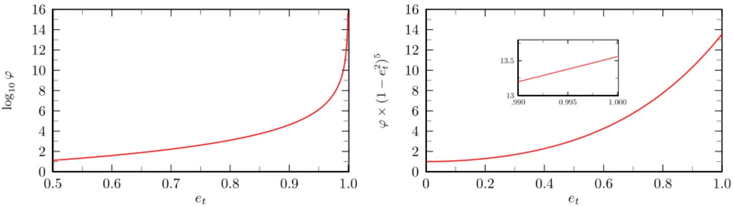
Only the leading terms are shown here; we have calculated over 100 terms withMathematica and presented part of this expansion previously (available online [82–84]). The first four terms are also published in [52]. The assumed singular factor turns out to be the correct one, allowing the remaining power series to converge to a finite value at et= 1. As can be seen from the rapidly diminishing size of higher-order terms, the series is convergent. The choice for singular factor is supported by asymptotic analysis found in Sec. IV C. The 1.5PN singular factor and the high-order expansion ofϕ(et) are two key results of this paper.
0 2 4 6 8 10 12 14 16
0.5 0.6 0.7 0.8 0.9 1.0
et
lo
g10
ϕ
0 2 4 6 8 10 12 14 16
0 0.2 0.4 0.6 0.8 1.0
et
ϕ
×
(1
−
e
2)t
5
13 13.5
.990 0.995 1.000
FIG. 2. Enhancement functionϕ(et) associated with the 1.5PN tail. On the left the enhancement function is directly plotted,
demonstrating the singular behavior aset→1. On the right, the eccentricity singular factor (1−e2t)−5 is removed to reveal
convergence in the remaining expansion to a finite value of approximately 13.5586 atet= 1.
2. Form of the 3PN Hereditary Terms
With a useful expansion of ϕ(et) in hand, we employ the same approach to the other hereditary terms. As a careful reading of Ref. [48] makes clear the most difficult contribution to calculate is (4.8), the correction of the 1.5PN tail showing up at 2.5PN order. Accordingly, we first consider the simpler 3PN case (4.9), which is the sum of the tail-of-the-tail and tail-squared terms [48]. The part in (4.9) that requires further investigation isχ(et). The infinite series forχ(et) is shown in [48] to be
χ(et) =1 4
∞
X
n=1
n2logn 2
g(n, et). (4.18)
The same technique as before is now applied toχ(et) using the expansion (4.15) ofg(n, et). The series will be singular at et= 1, so factoring out the singular behavior is important. However, for reasons to be explained in Sec. IV C, it proves essential in this case to remove the two strongest divergences. We find
χ(et) =−3
2F(et) log(1−e 2 t) +
1 (1−e2
t)13/2
(
−32 −773 log(2) +6561 256 log(3)
e2t (4.19)
+
−22 +34855
64 log(2)− 295245
1024 log(3)
e4t
+
−6595128 −1167467192 log(2) +24247269
16384 log(3) +
244140625 147456 log(5)
e6t
+
−31747768 +122348557
3072 log(2) +
486841509
131072 log(3)−
23193359375 1179648 log(5)
e8t+· · ·
)
.
Empirically, we found the series forχ(et) diverging like χ(et) ∼ −Cχ(1−e2t)−13/2log(1−e2t) as et→ 1, whereCχ is a constant. The first term in (4.19) apparently encapsulates all of the logarithmic divergence and implies that Cχ = −(3/2)(52745/1024) ' −77.2632. The reason for pulling out this particular function is based on a guess suggested by the asymptotic analysis in Sec. IV C and considerations on how logarithmically divergent terms in the combined instantaneous-plus-hereditary 3PN flux should cancel when a switch is made from orbital parametersetand yto parametersetand 1/p(to be further discussed in a forthcoming paper). Having isolated the two divergent terms, the remaining series converges rapidly with n. The divergent behavior of the second term aset→1 is computed to be approximately '+73.6036(1−e2t)−13/2. The appearance ofχ(et) is shown in Fig. 3, with and without its most singular factor removed.
3. Form of the 2.5PN Hereditary Term
0 5 10 15 20 25 30
0.2 0.3 0.4 0.5 0.6 0.7 0.8 0.9 1.0 et
lo
g10
χ
0 20 40 60 80 100
0 0.2 0.4 0.6 0.8 1.0
et
χ
/
si
n
g
.
fa
ct
o
r
70 80 90 100
0.990 0.995 1.000
FIG. 3. The 3PN enhancement functionχ(et). Its log is plotted on the left. On the right we remove the dominant singular
factor−(1−e2
t)−13/2log(1−e2t). The turnover nearet= 1 reflects competition with the next-most-singular factor, (1−e2t)−13/2.
0 3 6 9 12 15 18
0.5 0.6 0.7 0.8 0.9 1.0
et
lo
g10
|
ψ
|
−70 −60 −50 −40 −30 −20 −10 0
0 0.2 0.4 0.6 0.8 1.0
et
ψ
×
(1
−
e
2)t
6
−60
−58
−56
.990 0.995 1.000
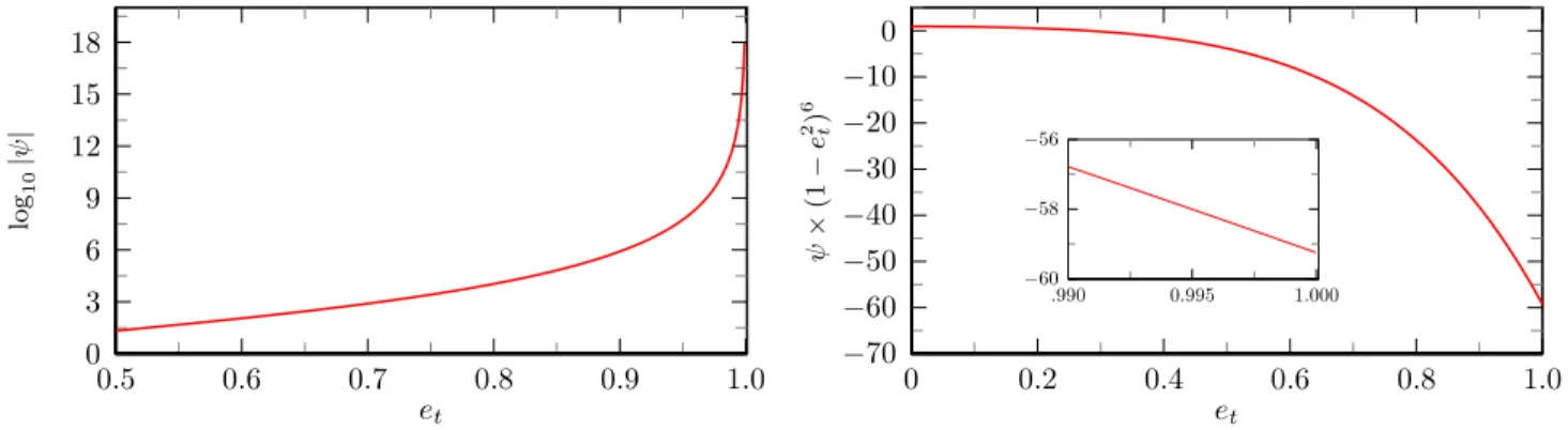
FIG. 4. The enhancement factor ψ(et). On the right we remove the singular factor (1−e2t)−6 and see the remaining
contribution smoothly approach a finite value atet= 1.
order the orbital motion no longer closes and the corrections in the mass quadrupole moments require a biperiodic Fourier expansion. Arun et al. [49] describe a procedure for computingψ, which they evaluated numerically. One of the successes we are able to report in this paper is having obtained a high-order power series expansion forψ in et. Even with Mathematica’s help, it is a consuming calculation, and we have reached only the 35th order (e70
t ). This achieves some of our purposes in seeking the expansion. We were also able to predict the comparable singular factor present aset→1 and demonstrate apparent convergence in the remaining series to a finite value atet= 1. The route we followed in making the calculation of the 2.5PN tail is described in App. A. Here, we give the first few terms in theψexpansion
ψ(et) = 1 (1−e2
t) 6
1−72134 8191e
2 t−
19817891 524224 e
4 t−
62900483 4718016 e
6 t−
184577393 603906048e
8 t+
1052581 419379200e
10 t
−1159499612160686351417 e12t +
106760742311 852232214937600e
14 t +
7574993235161 436342894048051200e
16 t
−25245553155637248004345876114169 e18t −
61259745206138959 56550039068627435520000e
20 t +· · ·
, (4.20)
Like in the preceding plots, we show log10|ψ|graphed on the left in Fig. 4. The singular behavior is evident. On the right side, the 2.5PN singular factor has been removed and the finite limit atet= 1 is clear.
C. Applying asymptotic analysis to determine eccentricity singular factors
at et= 1. We show now that at least some of these singular factors, specifically the ones associated withϕ(et) and χ(et), can be derived via asymptotic analysis. In the process the same analysis confirms the singular factors inf(et) andF(et) already known from post-Newtonian work. As a bonus our asymptotic analysis can even be used to make
remarkably sharp estimates of the limiting constant coefficients that multiply these singular factors.
What all four of these enhancement functions share is dependence on the square of the harmonics of the quadrupole moment given by the functiong(n, et) found in (4.12). To aid our analysis nearet= 1, we definex≡1−e2t and use xto rewrite (4.12) as
g(n, et) = 1 6n
21 +x+x2+ 3n2x3
(1−x)2 Jn(net) 2+1
2n
2x(1 +n2x) 1−x J
0
n(net)2−1 2n
3x(1 + 3x)
(1−x)3/2Jn(net)Jn0(net). (4.21) An inspection of how (4.21) folds into (4.11), (4.13), (4.14), and (4.18) shows that infinite sums of the following forms are required to computeϕ(et),χ(et),f(et), andF(et)
H0α,β= ∞
X
n=1
nαlogβn 2
Jn(net)2, H1α,β = ∞
X
n=1
nαlogβn 2
Jn0(net)2, H2α,β = ∞
X
n=1
nαlogβn 2
Jn(net)Jn0(net). (4.22) In this compact shorthand, β = 1 merely indicates sums that contain logs needed to calculate χ(et) while β = 0 (absence of a log) covers the other cases. Careful inspection of (4.21) reveals there are 18 different sums needed to calculate the four enhancement functions in question, andαranges over (some) values between 2 and 6.
As x→ 0 (et → 1) large n terms have growing importance in the sums. In this limit the Bessel functions have uniform asymptotic expansions for large ordernof the form [85–87]
Jn(net)∼
4ζ
x
1 4 "
n−1/3Ai(n2/3ζ) ∞
X
k=0 Ak n2k +n
−5/3Ai0(n2/3ζ) ∞ X k=0 Bk n2k # , (4.23)
Jn0(net)∼ −√ 2 1−x
x 4ζ
1 4"
n−4/3Ai(n2/3ζ) ∞
X
k=0 Ck n2k +n−
2/3Ai0(n2/3ζ) ∞ X k=0 Dk n2k # , (4.24)
whereζ depends on eccentricity and is found from 2
3ζ
3/2= log1 +√x √
1−x
−√x≡ρ(x)' 1 3x
3/2+1 5x
5/2+1 7x
7/2+
· · ·, (4.25)
and where the expansion ofρ(x) is the Puiseux series. Definingξ≡nρ(x), we need in turn the asymptotic expansions of the Airy functions [85–87]
Ai(n2/3ζ)∼ e− ξ
25/631/6√πξ1/6
1− 5 72ξ+
385 10368ξ2 −
85085 2239488ξ3 +
37182145 644972544ξ4 −
5391411025 46438023168ξ5 +· · ·
, (4.26)
Ai0(n2/3ζ)∼ −3
1/6ξ1/6e−ξ 27/6√π
1 + 7 72ξ−
455 10368ξ2+
95095 2239488ξ3 −
40415375 644972544ξ4 +
5763232475 46438023168ξ5 +· · ·
. (4.27)
In some of the following estimates all six leading terms in the Airy function expansions are important, while a careful analysis reveals that we never need to retain any terms in the Bessel function expansions beyondA0= 1 andD0= 1. These asymptotic expansions can now be used to analyze the behavior of the sums in (4.22) (from whence follow the enhancement functions) in the limit aset→1. Take as an example H23,0. We replace the Bessel functions with their asymptotic expansions and thus obtain an approximation for the sum
H23,0= ∞
X
n=1
n3Jn(net)Jn0(net)' 1 2π√1−x
∞
X
n=1 n2e−2ξ
1 + 1 36ξ−
35
2592ξ2 +· · ·
, (4.28)
where recall thatξis the product ofnwithρ(x). The original sum has in fact a closed form that can be found in the appendix of [78]
∞
X
n=1
n3Jn(net)Jn0(net) = et 4(1−e2
t)9/2
1 + 3e2t+ 3 8 e
4 t
∼3532 (1 1 −e2
t)9/2 '
1.094 (1−e2
t)9/2
where in the latter part of this line we give the behavior nearet= 1. With this as a target, we take the approximate sum in (4.28) and make a further approximation by replacing the sum over n with an integral overξ from 0 to∞ while letting ∆n= 1→ dξ/ρ(x) and retaining only terms in the expansion that yield non-divergent integrals. We find
1 2π√1−x
1 ρ(x)3
Z ∞
0
dξ e−2ξ
ξ2+ 1 36ξ−
35 2592
= 1297 10368π
1
ρ(x)3√1−x ∼ 1297 384π
1 (1−e2
t)9/2 '
1.0751 (1−e2
t)9/2
, (4.30)
with the final result coming from further expanding in powers of x. Our asymptotic calculation, and approximate replacement of sum with integral, not only provides the known singular dependence but also an estimate of the coefficient on the singular term that is better than we perhaps had any reason to expect.
All of the remaining 17 sums in (4.22) can be approximated in the same way. As an aside it is worth noting that for those sums in (4.22) without log terms (i.e.,β= 0) the replacement of the Bessel functions with their asymptotic expansions leads to infinite sums that can be identified as the known polylogarithm functions [86, 87]
Li−k
e−2ρ(x)= ∞
X
n=1
nke−2nρ(x). (4.31)
However, expanding the polylogarithms as x→ 0 provides results for the leading singular dependence that are no different from those of the integral approximation. Since theβ = 1 cases are not represented by polylogarithms, we simply uniformly use the integral approximation.
We can apply these estimates to the four enhancement functions. First, the Peters-Mathews functionf(et) in (4.11) has known leading singular dependence of
f(et)'
1 + 73 24+
37 96
1 (1−e2
t)7/2 = 425
96 1 (1−e2
t)7/2 '
4.4271 (1−e2
t)7/2
, as et→1. (4.32)
If we instead make an asymptotic analysis of the sum in (4.11) we find
f(et)∼
191755 13824π
1 (1−e2
t)7/2 '
4.4153 (1−e2
t)7/2
, (4.33)
which extracts the correct eccentricity singular function and yields a surprisingly sharp estimate of the coefficient. We next turn to the functionF(et) in (4.13). In this case the function tends toF(et)'(52745/1024)(1−e2t)−13/2' 51.509(1−e2
t)−13/2 aset→1. Using instead the asymptotic technique we get an estimate F(et)∼
5148642773 31850496π
1 (1−e2
t)13/2 '
51.455 (1−e2
t)13/2
. (4.34)
Once again the correct singular function emerges and a surprisingly accurate estimate of the coefficient is obtained. These two cases are heartening checks on the asymptotic analysis but of course both functions already have known closed forms. What is more interesting is to apply the approach toϕ(et) andχ(et), which are not known analytically. For the sum in (4.14) forϕ(et) we obtain the following asymptotic estimate
ϕ(et)∼
56622073 1327104π
1 (1−e2
t)5 −
371833517 6635520π
1 (1−e2
t)4
+· · · ' 13.581 (1−e2
t)5 −
17.837 (1−e2
t)4
+· · ·, (4.35)
where in this case we retained the first two terms in the expansion about et = 1. The leading singular factor is exactly the one we identified in IV B 1 and its coefficient is remarkably close to the 13.5586 value found by numerically evaluating the high-order expansion in (4.17). The second term was retained merely to illustrate that the expansion is a regular power series inxstarting withx−5(in contrast to the next case).
We come finally to the enhancement function, χ(et), whose definition (4.18) involves logarithms. Using the same asymptotic expansions and integral approximation for the sum, and retaining the first two divergent terms, we find
χ(et)∼ −
5148642773 21233664π
log(1−e2 t) (1−e2
t)13/2−
5148642773 21233664π
−78824531645148642773+2 3γE+
4
3log(2)− 2 3log(3)
1
(1−e2 t)13/2
. (4.36)
The form of (4.19) assumed in Sec. IV B 2, whose usefulness was verified through direct high-order expansion, was suggested by the leading singular behavior emerging from this asymptotic analysis. We guessed that there would be two terms, one with eccentricity singular factor log(1−e2
made close toet= 1 these two leading terms compete with each other, with the logarithmic term only winning out slowly as et→1. Prior to identifying the two divergent series we initially had difficulty with slow convergence of an expansion forχ(et) in which only the divergent term with the logarithm was factored out. To see the issue, it is useful to numerically evaluate our approximation (4.36)
χ(et)∼ −77.1823
log(1−e2 t) (1−e2
t)13/2
1− 0.954378 log(1−e2 t)
=−77.1823log(1−e 2 t) (1−e2
t)13/2
+ 73.6612 (1−e2
t)13/2
. (4.37)
From this it is clear that even atet= 0.99 the second term makes a +24.3% correction to the first term, giving the misleading impression that the leading coefficient is near −96 not−77. The key additional insight was to guess the closed form for the leading singular term in (4.19). As mentioned, the reason for expecting this exact relationship comes from balancing and cancelling logarithmic terms in both instantaneous and hereditary 3PN terms when the expansion is converted from one inetandyto one inetand 1/p. The coefficient on the leading (logarithmic) divergent term inχ(et) is exactly −(3/2)(52745/1024)' −77.2632. [This number is -3/2 times the limit of the polynomial in F(et).] It compares well with the first number in (4.37). Additionally, recalling the discussion made following (4.19), the actual coefficient found on the (1−e2
t)−13/2 term is +73.6036, which compares well with the second number in (4.37). The asymptotic analysis has thus again provided remarkably sharp estimates for an eccentricity singular factor. 1
D. Using Darwin eccentricityeto map I(et) and K(et) toI˜(e)and K˜(e)
Our discussion thus far has given the PN energy flux in terms of the standard QK time eccentricityetin modified harmonic gauge [50]. The motion is only known presently to 3PN relative order, which means that the QK repre-sentation can only be transformed between gauges up to and includingy3 corrections. At the same time, our BHP calculations accurately include all relativistic effects that are first order in the mass ratio. It is possible to relate the relativistic (Darwin) eccentricitye to the QK et (in, say, modified harmonic gauge) up through correction terms of ordery3,
e2 t
e2 =1−6y−
15−19√1−e2+ 15√1−e2−15e2
(1−e2)3/2 y
2
+ 1
(1−e2)5/2
30−38p1−e2+59p1−e2−75e2+45
−18p1−e2e4
y3. (4.38)
See [50] for the low-eccentricity limit of this more general expression. We do not presently know how to calculateet beyond this order. Using this expression we can at least transform expected fluxes to their form in terms ofe and check current PN results through 3PN order. However, to go from 3PN to 7PN, as we do in this paper, our results must be given in terms ofe.
The instantaneous (I) and hereditary (K) flux terms may be rewritten in terms of the relativistic eccentricity e straightforwardly by substitutingeforetusing (4.38) in the full 3PN flux (4.1) and re-expanding the result in powers ofy. All flux coefficients that are lowest order iny are unaffected by this transformation. Instead, only higher order corrections are modified. We find
˜
I0(e) =I0(et), K˜3/2(e) =K3/2(et), K˜3(e) =K3(et), (4.39) ˜
I1(e) = 1 (1−e2)9/2
−1247336 −15901672 e2
−9253384 e4
−40371792e6
, (4.40)
˜ I2(e) =
1 (1−e2)11/2
−2034719072 −143087318144 e2+2161337 24192 e
4+231899 2304 e
6+499451 64512 e
8 (4.41)
+ 1
(1−e2)5
35
2 + 1715
48 e 2
−297564 e4−1295 192 e
6, ˜
I3(e) = 1 (1−e2)13/2
2193295679
9979200 +
55022404229 19958400 e
2+68454474929 13305600 e
4 (4.42)
1 Note added in proof: while this paper was in press the authors
+40029894853 26611200 e
6
−32487334699141926400 e8−23374565311354112e10
+ 1
(1−e2)6
−14047483151200 −75546769100800 e2
−210234049403200 e4+1128608203 2419200 e
6+617515 10752 e
8
+1712 105 log
"
y y0
1 +√1−e2 2(1−e2)
#
F(e),
˜
K5/2(e) = − π (1−e2)6
8191
672 + 62003
336 e
2+20327389 43008 e
4+87458089 387072 e
6+67638841 7077888e
8+ 332887 25804800e
10
−475634073600482542621 e12+ 43302428147 69918208819200e
14
−357981229154304002970543742759 e16 + 3024851376397
207117711153561600e
18+ 24605201296594481 4639436729839779840000e
20+ · · ·
, (4.43)
whereF is given by (4.6) withet→e. The full 3PN flux is written exactly as Eqn. (4.1) withI →I˜ andK →K˜.
V. CONFIRMING ECCENTRIC-ORBIT FLUXES THROUGH 3PN RELATIVE ORDER
Sections II and III briefly described a formalism for an efficient, arbitrary-precision MST code for use with eccentric orbits. Section IV detailed new high-order expansions in e2 that we have developed for the hereditary PN terms. The next goal of this paper is to check all known PN coefficients for the energy flux (at lowest order in the mass ratio) for eccentric orbits. The MST code is written inMathematica to allow use of its arbitrary precision functions. Like previous circular orbit calculations [27, 28], we employ very high accuracy calculations (here up to 200 decimal places of accuracy) on orbits with very wide separations (p'1015
−1035). Why such wide separations? Atp= 1020, successive terms in a PN expansion separate by 20 decimal places from each other (10 decimal places for half-PN order jumps). It is like doing QED calculations and being able to dial down the fine structure constant from α'1/137 to 10−20. This in turn mandates the use of exceedingly high-accuracy calculations; it is only by calculating with 200 decimal places that we can observe∼10 PN orders in our numerical results with some accuracy.
A. Generating numerical results with the MST code
In Secs. II and III we covered the theoretical framework our code uses. We now provide an algorithmic roadmap for the code. (While the primary focus of this paper is in computing fluxes, the code is also capable of calculating local quantities to the same high accuracy.)
• Solve orbit equations for given p ande. Given a set of orbital parameters, we findtp(χ), ϕp(χ), and rp(χ) to high accuracy at locations equally spaced in χ. We do so by employing the SSI method outlined in Sec. II B of Ref. [56]. From these functions we also obtain the orbital frequencies Ωr and Ωϕ. All quantities are computed with some pre-determined overall accuracy goal; in this paper it was a goal of 200 decimal places of accuracy in the energy flux.
• Obtain homogeneous solutions to the FD RWZ master equation for given lmnmode. We find the homogeneous solutions using the MST formalism outlined in Sec. II B. The details of the calculation are given here.
1.Solve for ν. For eachlmn, theω-dependent renormalized angular momentumν is determined (App. B). 2.Determine at what n to truncate infinite MST sums involvingan. The solutionsRup/inlmω are infinite sums
3.Evaluate Teukolsky function between rmin andrmax. Using the truncation of the infinite MST series, we evaluateRup/inlmω and their first derivative [higher derivatives are found using the homogeneous differential equation (2.3)] at therlocations corresponding to the even-χspacing found in Step 1. The high precision evaluation of hypergeometric functions in this step represents the computational bottleneck in the code. 4.Transform Teukolsky function to RWZ master functions. Forl+modd we use Eqn. (2.15) to obtain ˆXlmn± .
Whenl+mis even we continue and use Eqn. (2.16).
5.Scale master functions. In solving for the fluxes, it is convenient to work with homogeneous solutions that are unit-normalized at the horizon and at infinity. We divide the RWZ solutions by the asymptotic amplitudes that arise from choosing a0 = 1 when forming the MST solutions to the Teukolsky equation. These asymptotic forms are given in Eqns. (2.17)-(2.19).
• Formlmn flux contribution. Form Clmn+ using the exponentially-convergent SSI sum (3.24). Note that this ex-ponential convergence relies on the fact that we evaluated the homogeneous solutions at evenly-spaced locations in χ. The coefficientClmn+ feeds into a single positive-definite term in the sum (3.25).
• Sum overlmn modes. In reconstructing the total flux there are three sums:
1.Sum overn. For each spherical harmoniclm, there is formally an infinite Fourier series sum fromn=−∞ to∞. In practice the SSI method shows thatnis effectively bounded in some range−N1≤n≤N2. This range is determined by the fineness of the evenly-spaced sampling of the orbit in χ. For a given orbital sampling, we sum modes between−N1≤n≤N2, whereN1 and N2 are the first Nyquist-like notches in frequency, beyond which aliasing effects set in [56].
2.Sum over m. For eachl mode, we sum overmfrom−l≤m≤l. In practice, symmetry allows us to sum from 0≤m≤l, multiplying positivemcontributions by 2.
3.Sum over l. The sum overl is, again, formally infinite. However, each multipole order appears at a higher PN order, the spacing of which depends on 1/p. The leadingl= 2 quadrupole flux appears atO(p−5). For an orbit withp= 1020, thel= 3 flux appears at a level 20 orders of magnitude smaller. Only contributions through l ≤12 are necessary with this orbit and an overall precision goal of 200 digits. This cutoff inl varies with differentp.
B. Numerically confirming eccentric-orbit PN results through 3PN order
We now turn to confirming past eccentric-orbit PN calculations. The MST code takes as input the orbital parameters pand e. Then 1/pis a small parameter. Expandingdtp/dχin (3.5) we find from (3.6)
Ωr= 1 M
1
−e2 p
3/2(
1−31−e 2
p −
3 2
√
1−e2[5−2√1−e2+e2(
−5 + 6√1−e2)]
p2 +· · ·
)
. (5.1)
Expanding (3.8) in similar fashion gives
Ωϕ= 1 M
1
−e2 p
3/2( 1 + 3e
2 p −
3 4
10(−1 +√1−e2) +e2(20
−3√1−e2) + 2e4(
−5 + 6√1−e2) √
1−e2p2 +· · ·
)
. (5.2)
Then given the definition ofy we obtain an expansion ofy in terms ofp
y= 1−e 2
p +
2e2(1 −e2)
p2 +
1 2
p
1−e2
10(1−√1−e2) +e2(
−3 + 10√1−e2) + 10e4)
p3 +· · · . (5.3)
So from our chosen parameters e and pwe can obtain y to arbitrary accuracy, and then other orbital parameters, such as Ωrand Ωϕ, can be computed as well to any desired accuracy.
−300 −250 −200 −150 −100
-100 -50 0 50 100
log
D ˙E
∞ `mn
E
Harmonic numbern
FIG. 5. Fourier-harmonic energy-flux spectra from an orbit with semi-latus rectum p = 1020 and eccentricity e = 0.1. Each inverted-V spectrum represents flux contributions of modes with various harmonic numbern but fixed l and m. The tallest spectrum traces the harmonics of the l = 2, m = 2 quadrupole mode, the dominant contributor to the flux. Spectra of successively higher multipoles (octupole, hex-adecapole, etc) each drop 20 orders of magnitude in strength as lincreases by one (l ≤12 are shown). Every flux contri-bution is computed that is within 200 decimal places of the peak of the quadrupole spectrum. Withe= 0.1, there were 7,418 significant modes that had to be computed (and are shown above).
−80 −70 −60 −50 −40 −30 −20 −10 0 10
0 0.02 0.04 0.06 0.08 0.1
log
(PN
res
idual
s)
eccentricitye Peters-Mathews Flux
hE˙i −Peters-Mathews =O(1PN)
hE˙i −1PN =O(1.5PN)
hE˙i −1.5PN =O(2PN)
hE˙i −2PN =O(2.5PN)
hE˙i −2.5PN =O(3PN)
hE˙i −3PN =O(3.5PN)
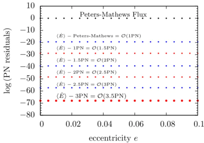
FIG. 6. Residuals after subtracting from the numerical data successive PN contributions. Residuals are shown for a set of orbits with p = 1020 and a range of eccentricities from
e = 0.005 through e = 0.1 in steps of 0.005. Residuals are scaled relative to the Peters-Mathews flux (uppermost points at unit level). The next set of points (blue) shows residu-als after subtracting the Peters-Mathews enhancement from BHP data. Residuals drop uniformly by 20 order of magni-tude, consistent with 1PN corrections in the data. The next (red) points result from subtracting the 1PN term, giving residuals at the 1.5PN level. Successive subtraction of known PN terms is made, reaching final residuals at 70 orders of magnitude below the total flux and indicating the presence of 3.5PN contributions in the numerical fluxes.
Next, we compute the PN parts of the expected flux using Eqns. (4.39) through (4.43). The predicted fluxF3PN is very close to the computed fluxFMST. We then subtract the quadrupole theoretical flux term
FN= 32 5
µ
M
2
y5I˜0(e)≡ FNcirc I˜0(e), (5.4)
from the flux computed with the MST code (and normalize with respect to the Newtonian term)
FMST− FN FN
=O(y)' ˜1 I0(e)
h
yI˜1(e) +y3/2K˜3/2(e) +y2I˜2(e) +y5/2K˜5/2(e) +y3I˜3(e) +y3K˜3(e)
i
, (5.5)
and find a residual that is 20 orders of magnitude smaller than the quadrupole flux. The residual reflects the fact that our numerical (MST code) data contains the 1PN and higher corrections. We next subtract the 1PN term
FMST− FN
FN −
yI˜˜1(e) I0(e)
=O(y3/2), (5.6)
and find residuals that are another 10 orders of magnitude lower. This reflects the expected 1.5PN tail correction. Using our high-order expansion forϕ(e), we subtract and reach 2PN residuals. Continuing in this way, once the 3PN term is subtracted, the residuals lie at a level 70 orders of magnitude below the quadrupole flux. We have reached the 3.5PN contributions, which are encoded in the MST result but whose form is (heretofore) unknown. Fig. 6 shows this process of successive subtraction. We conclude that the published PN coefficients [10, 48]for eccentric orbits in the lowest order inν limit are all correct. Any error would have to be at the level of one part in 1010 (and only then in the 3PN terms) or it would show up in the residuals.
![FIG. 8. Strong-field comparison between the 7PN expansion and energy fluxes computed with a Lorenz gauge/RWZ gauge hybrid self-force code [93] (courtesy T](https://thumb-us.123doks.com/thumbv2/123dok_us/8274277.2191352/23.918.104.448.113.351/strong-comparison-expansion-energy-fluxes-computed-lorenz-courtesy.webp)